This tutorial is part of the Pivot Table Formatting, Output & Special Behavior in Google Sheets hub, where we cover advanced Pivot Table behavior, limitations, and reliable workarounds.
If you’re trying to extract subtotal rows or the grand total row from a Pivot Table in Google Sheets, you’ve probably discovered a major limitation:
👉 GETPIVOTDATA cannot dynamically return entire total rows.
In this guide, you’ll learn a simple, fully dynamic formula that extracts all subtotal rows and the grand total row—even when the Pivot Table layout changes.
Why GETPIVOTDATA Fails for Total Rows
The GETPIVOTDATA function works well when you want to retrieve individual aggregated values from a Pivot Table.
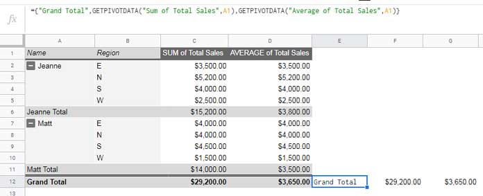
For example, this formula successfully extracts the grand total row values:
={"Grand Total",
  GETPIVOTDATA("Sum of Total Sales",A1),
  GETPIVOTDATA("Average of Total Sales",A1)
}
Why the Real Problem Starts With Subtotals
If your Pivot Table includes subtotal rows like:
- Jeanne Total
- Matt Total
- Grand Total
You must manually nest a separate GETPIVOTDATA call for every subtotal row:
={
 "Jeanne Total",
 GETPIVOTDATA("Sum of Total Sales",A1,"Name","Jeanne"),
 GETPIVOTDATA("Average of Total Sales",A1,"Name","Jeanne");
 {"Matt Total",
 GETPIVOTDATA("Sum of Total Sales",A1,"Name","Matt"),
 GETPIVOTDATA("Average of Total Sales",A1,"Name","Matt")};
 {"Grand Total",
 GETPIVOTDATA("Sum of Total Sales",A1),
 GETPIVOTDATA("Average of Total Sales",A1)}
}
🚫 This is not dynamic.
Every new category or subtotal requires manual editing.
The Better Solution: Extract Total Rows Dynamically
Instead of fighting GETPIVOTDATA, you can directly filter the Pivot Table output.
Dynamic Formula to Extract Subtotal and Grand Total Rows
=FILTER(A1:D, SEARCH("Total", A1:A) > 1)
What the Formula Does
- Scans column A of the Pivot Table
- Identifies rows containing the word “Total”
- Returns all subtotal rows + the grand total row
- Automatically updates when:
- New categories are added
- Row order changes
- Pivot Table expands or contracts
Example Output (Subtotal and Grand Total Rows)
| Name | Sum of Sales | Average Sales |
|---|---|---|
| Jeanne Total | 15,200 | 3,800 |
| Matt Total | 14,000 | 3,500 |
| Grand Total | 29,200 | 3,650 |
No nesting, no hardcoding, and no ongoing maintenance required.
Why This Method Is Truly Dynamic
Assume you add a new employee—Alex—to the source data.
Once the Pivot Table refreshes:
- A new “Alex Total” row appears
- The formula automatically includes it
- No edits required
That’s what dynamic extraction of total rows from a Pivot Table actually means.
How the FILTER + SEARCH Combo Works
FILTER Syntax Refresher
FILTER(range, condition)
In this case:
- range →
A1:D(entire Pivot Table output) - condition → rows that contain
"Total"
Why SEARCH Is Required
FILTER does not support wildcard matching like "*Total*".
So instead, we use:
SEARCH("Total", A1:A) > 1
- SEARCH returns a number when text is found
- That numeric result becomes the filter condition
- Rows without
"Total"are excluded
This makes the formula both flexible and reliable.
Common Questions
Can I Extract Only the Grand Total Row?
Yes. If your Pivot Table labels the row as "Grand Total", replace "Total" with "Grand Total" in the formula.
Will This Work If the Pivot Table Moves?
Yes. As long as the referenced range includes the Pivot Table output.
Does This Work With Multiple Value Columns?
Yes. The formula scales automatically across columns.
When You Should NOT Use This Method
- If you need individual aggregated values tied to field names
- If the Pivot Table is set to hide subtotal labels
- If your totals don’t include consistent text like
"Total"
In those cases, GETPIVOTDATA may still be appropriate.
Final Thoughts
If your goal is to extract subtotal and grand total rows from a Pivot Table in Google Sheets, this FILTER + SEARCH method is:
- Cleaner than GETPIVOTDATA
- Fully dynamic
- Easy to audit
- Future-proof against layout changes
👉 For related techniques, see the hub section on Pivot Table Calculations & Advanced Metrics.
Related Resources
If you want to go deeper into advanced Pivot Table formulas and understand when GETPIVOTDATA is still the right tool, check out these related guides:
Using GETPIVOTDATA with Grouped Dates in Google Sheets – A practical guide to extracting values from Pivot Tables that use grouped date fields (months, quarters, years).
Unlock the Power of GETPIVOTDATA Arrays in Google Sheets – Learn how to work with array-style GETPIVOTDATA formulas and when they outperform traditional approaches.


