Adding a Calculated Field in a Pivot Table in Google Sheets

You may have noticed the option to add a Calculated field under the Values section of a pivot table in Google Sheets. But when should you actually use it, and how does it differ from standard pivot table calculations?

In this tutorial, you’ll learn when and where to use calculated fields in Google Sheets pivot tables, along with a practical example you can adapt to real-world reports.

Table of Contents

When Do You Need a Calculated Field?

Most pivot table summaries don’t require custom formulas. Google Sheets already provides built-in aggregation functions such as:

SUM
COUNT
MAX
MIN
AVERAGE

These functions are sufficient for basic grouping and summarization.

However, calculated fields become necessary when your logic depends on derived or custom calculations, such as:

Using the most recent value instead of MAX or AVERAGE
Multiplying two aggregated results
Applying conditional or lookup-based logic inside a pivot table

That’s where calculated fields truly shine.

Example Use Case

In this example, we’ll summarize material sales and calculate the most recent price per unit for each material — something that standard pivot table functions can’t do on their own.

This article is part of the Pivot Table Calculations & Advanced Metrics in Google Sheets hub, which explores advanced pivot reporting techniques.

Sample Dataset Overview

Our source data includes:

Date
Material name
Number of units
Price per unit

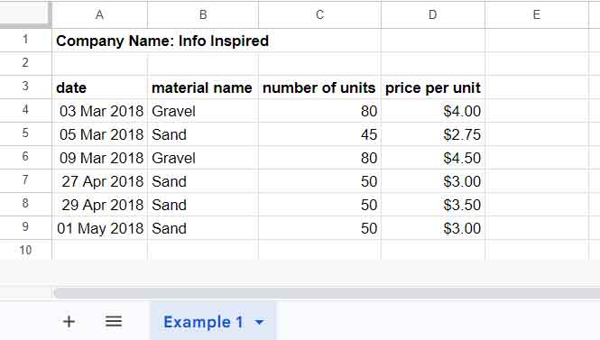
Sample source data used for adding a calculated field in a Google Sheets pivot table

This simple dataset helps demonstrate how calculated fields work inside a pivot table.

You’ll find a sample Google Sheets file at the end of this post to follow along or review the final result.

Step 1: Prepare the Pivot Table

Select the source range A3:D9
Go to Insert → Pivot table
(Earlier, this option was under the Data menu.)
Choose New sheet, then click Create

This opens the Pivot table editor panel.

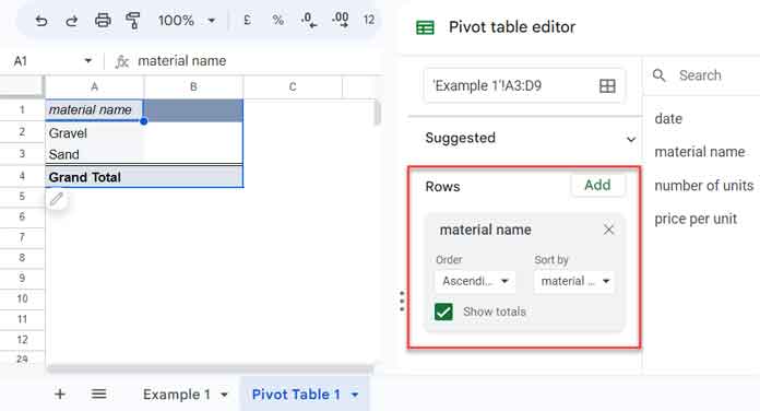
Grouping Rows

To group the data by material:

Click Add next to Rows
Select material name

This groups the report by items such as Gravel and Sand.

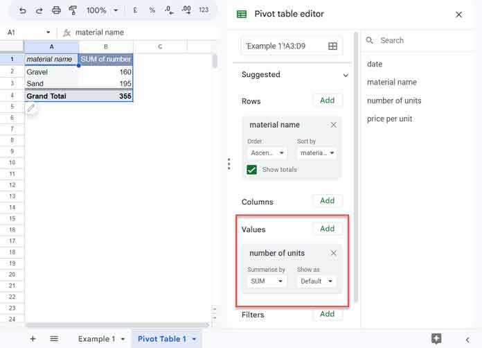
Grouping rows by material name in a Google Sheets pivot table

Adding a Quantity Column

To calculate total quantity:

Click Add next to Values
Select number of units
Under Summarize by, choose SUM

At this point, your pivot table shows:

Material name
Total number of units sold

Now you’re ready to add a calculated field.

Summing values in the Values section of a Google Sheets pivot table

Step 2: Add a Calculated Field for the Most Recent Price

Here’s the challenge:

Each material has different prices on different dates
Using MAX, MIN, or AVERAGE for price would give misleading results
We want the most recent price per unit instead

Important Prerequisite

The source data must be sorted by date:

Ascending order → use one formula
Descending order → use a slightly modified version

(This example assumes ascending order.)

Adding the Calculated Field

In the Pivot table editor, click Add next to Values
Select Calculated field
Remove the default formula =0
Set Summarize by to Custom
Enter the following formula:

=XLOOKUP('material name','material name','price per unit',,0,-1)

Click outside the formula field to apply it.

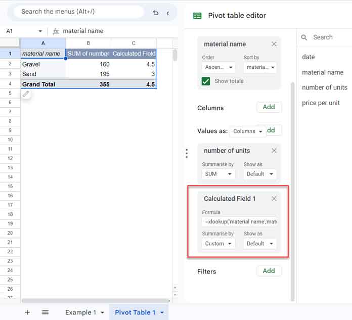
Adding a calculated field to the Values section in a Google Sheets pivot table

This XLOOKUP formula searches for each material name in the source data and returns the last matching price per unit, which corresponds to the most recent price.

The -1 search mode instructs XLOOKUP to search from the bottom of the dataset upward, ensuring the latest value is returned when the source data is sorted by date.

At this point, the pivot table includes a calculated field that shows the most recent price per unit for each material.

Any changes to the source data will automatically update this value.

Step 3: Calculate the Total Amount (Quantity × Recent Price)

To calculate the total amount:

Add another Calculated field
Use this formula:

=SUM('number of units') * XLOOKUP('material name','material name','price per unit',,0,-1)

This formula multiplies the aggregated total quantity from the pivot table with the most recent price per unit retrieved from the source data.

SUM('number of units') returns the total quantity for each grouped material, while the XLOOKUP expression fetches the latest corresponding price based on the sorted date order.

Calculated field formulas to get the most recent price and total amount in a Google Sheets pivot table

The result is the total amount calculated using the most up-to-date price.

If Your Data Is Sorted in Descending Order

Replace -1 with 1 in both formulas.

Things to Remember When Writing Calculated Field Formulas

Keep these rules in mind:

Always reference source fields, not pivot table cells
Use field labels, not ranges
- Example: 'price per unit', not D4:D9
Enclose field labels in single quotes
Calculated fields operate on aggregated data, not row-level values

How to Rename a Calculated Field in Google Sheets

Calculated fields can’t be renamed from the editor panel.

Instead:

Click the column header cell in the pivot table
Manually overwrite it with your desired name
(For example, rename Calculated Field 1 to Price)

Final Thoughts

Calculated fields allow you to perform advanced logic directly inside pivot tables, without modifying your source data.

If you frequently work with:

Derived metrics
Lookup-based calculations
Aggregated formulas

Calculated fields are an essential tool.

Thanks for reading — and enjoy building smarter pivot table reports!

Sample Sheet

14 COMMENTS

Arelis July 29, 2025 At 2:59 am

Hi,

I’m trying to create a calculated value in a pivot table. I’m attempting to sum and count the value of ticket revenue, but the formula is giving me an error. I’ve enclosed the text in single quotes, but it still doesn’t work. This is the formula I have:
=SUMA('Ingresos en taquilla ($)')/CONTAR('Ingresos en taquilla ($)')

What can I do?

- Prashanth KV July 29, 2025 At 8:45 am
  
  Hi Arelis,
  
  Thanks for your question!
  
  It looks like you’re working with the Spanish version of Google Sheets. Please make sure the field name in your formula exactly matches the one in your source data, and that you’re using the correct function names in Spanish.
  
  For example:
  
  For example: =SUMA('Ingresos en taquilla ($)') / CONTAR('Ingresos en taquilla ($)')
  
  Also, be sure to use straight quotes (') instead of curly ones (‘’), as curly quotes can cause formula errors.
  
  That said, you may not need a calculated field for this. You can use the AVERAGE function directly within the pivot table to get the same result more easily.
  
  Hope this helps!
  
Grant September 25, 2022 At 7:06 pm

Is there a way to go about calculating the difference between to values columns in the pivot table?

I’ve tried something like =b4-d4, but the results (same number) apply to all cells in calculated field 1.

I want it to be unique and reflected across all rows. What am I doing wrong here? Thanks

- Prashanth September 26, 2022 At 12:09 pm
  
  Hi, Grant,
  
  That might be easy by adding an extra column to your source data.
  
  Feel free to share a sample sheet URL in the comment below.
  
Anushma Datt October 16, 2020 At 8:38 am

Hi, All,

I am trying to hide the Pivot Table Editor. So that I can view my Pivot Table. Any tips for this?

- Prashanth October 16, 2020 At 9:58 am
  
  Hi, Anushma Datt,
  
  You just click outside the Pivot Table output range. It will hide the editor. There is no other way, at least for now!
  
S K Srivastava May 25, 2020 At 9:03 am

Thanx. Sumproduct worked.

=sumproduct(Nur_type="Plants",Num_plants)

I was able to get the desired output following formula

=sum(arrayformula(if(nur_type="Plants",Num_plants,0)))

But it was too clumsy. Sumproduct is sleek.

Thanx once again.

S K Srivastava May 24, 2020 At 7:54 pm

I have noted that Sumif or Sumifs do not work in calculated field in the pivot table while Countif/Countifs work without any issue. I think there is some bug.

Can you please check and confirm.

- Prashanth May 25, 2020 At 8:28 am
  
  Hi, S K Srivastava,
  
  That’s possibly due to the last argument, i.e. sum_range.
  
  It may not be a bug associated with the Pivot Table. It’s most probably associated with the capability of the Sumif function.
  
  In your spreadsheet also, you will see the same issue with Sumif in some cases like when you are trying to use an expression as the sum_range.
  
  You may better use Sumproduct.
  
  For example, this Sumif can be replaced by;
  
  =sumif(zone,"north",qty)
  
  the below Sumproduct.
  
  =sumproduct(zone="north",qty)
  
  Best,
  
Joshua Seal May 1, 2020 At 7:14 am

I notice that the ‘Grand Total’ for each of the ‘Calculated Field’ columns are incorrect in your examples.

I’ve found this happens with my Calculated Field’s inside of pivot tables when I select ‘summarize by’ “custom”. Is this a bug in sheets, or is there some logic to it?

For me, sometimes the Grand Total looks like it just selects at random one of the results in the column above. Other times I’ve seen results that I can seem to explain.

- Joshua Seal May 1, 2020 At 9:31 am
  
  Did a little digging. It turns out that the ‘grand total’ row doesn’t always sum the values above it, but instead applies the function to all of the data in question. It’s a poor choice of wording.
  
  I was trying to get a sum of just the unique values, so I ended up creating a calculated field with the formula =sum(UNIQUE ('field name'))
  
- Prashanth May 1, 2020 At 4:24 pm
  
  Hi, Joshua Seal,
  
  The total is actually the multiplication of the values from the grand total row itself. Not the sum of the column.
  
  When using ‘Calculated Fields’ in Pivot Table reports disable the ‘Grand Total’ under row grouping within the editor. I think that would be better to avoid confusion.
  
  I’ve just included my sample pivot table sheet within the post (in the last part).
  
Kelvin December 31, 2018 At 6:31 am

Hello, This is great stuff. Thanks for sharing. Using the name of source field can be a little confusing instead of being able to just simply click on a cell. Wish it was that simple. With that said I have a question about calculated fields formula.

If I am trying to calculate impressions by grand total impressions (shown on the table) how do I go about doing so? For instance, =sum(Impr.)/1108. It works if I do use a specific number but how do I use contextual formulas to calculate this?

Thanks for your help.

- Jim November 15, 2022 At 12:45 pm
  
  Is there a possible answer to this?