Grouping dates in a Pivot Table in Google Sheets is a powerful way to create monthly, quarterly, and yearly summary reports. It helps you analyze trends in your data without needing formulas like QUERY or SUMIF, which can be tricky for beginners. Even a novice can quickly summarize data using this feature.
For example, suppose you track your day-to-day expenses in Google Sheets. By grouping the date column in a Pivot Table, you can easily see:
- How much you spend each month
- Which month had unusually high expenses
- Quarterly or yearly spending trends
This tutorial is part of our complete Google Sheets Pivot Table Tutorial, covering everything from basics to advanced date grouping techniques.
How to Group Dates in a Pivot Table in Google Sheets
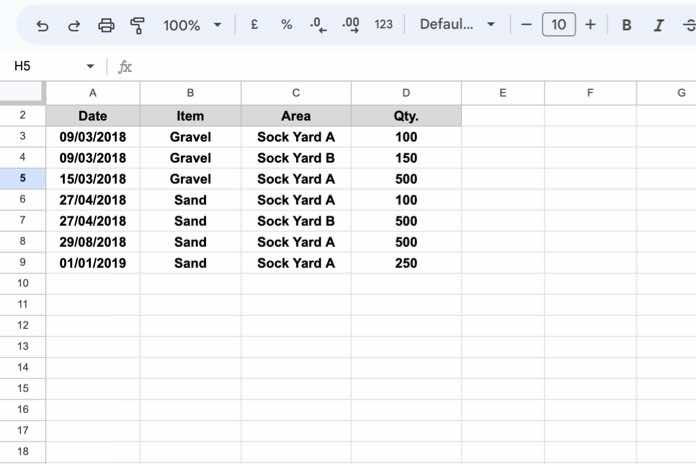
The sample data consists of Date, Item, Area, and Qty in columns A through D. It’s a very basic dataset designed to explain the core concept of date grouping. See the screenshot below.
Step 1: Create a Pivot Table
Start with your sample data in Google Sheets. Before grouping dates, you need a Pivot Table:
- Select your data range (e.g.,
A1:D9). - Go to the Insert menu → Pivot table.
- Choose where the Pivot Table should appear (new sheet or existing sheet). Click Create.
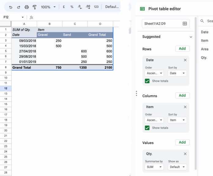
Google Sheets will create a new Pivot Table at the chosen location. If you selected a new sheet, a new tab (e.g., “Pivot Table 1”) will open. The Pivot Table editor panel will appear on the right, and the sheet will show a table skeleton ready for you to add Rows, Columns, and Values.
Step 2: Add Rows, Columns, and Values
Set up your Pivot Table:
- Rows: Date
- Columns: Item
- Values: Qty (Summarize by SUM)
Now, if any items repeat on the same date, their quantities will automatically sum, giving you an initial grouping.
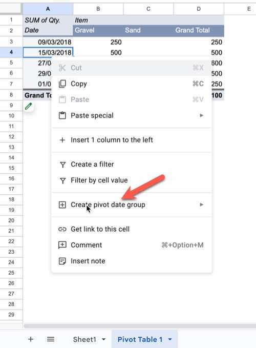
Step 3: Find the Date Grouping Option
Date grouping is not available in the Pivot Table editor panel—it’s hidden in the right-click shortcut menu:
- Go to a cell in the Pivot Table containing a date (e.g.,
A3:A7). - Right-click the cell → select Create pivot date group.
- You’ll see multiple options for grouping dates: Month, Year-Month, Quarter, Year-Quarter, or Year.
Step 4: Group by Month or Year-Month
- Month: Groups all dates by month, ignoring the year. For example, January 2018 and January 2019 are combined.
- Year-Month: Groups dates by both year and month, keeping January 2018 and January 2019 separate.
Tip: Use Year-Month if your data spans multiple years.
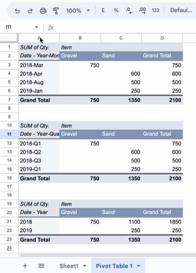
Step 5: Group by Quarter or Year-Quarter
Quarters are commonly used in financial reporting:
| Quarter | Months |
|---|---|
| Q1 | January – March |
| Q2 | April – June |
| Q3 | July – September |
| Q4 | October – December |
- Quarter: Groups months into quarters, ignoring the year.
- Year-Quarter: Groups quarters by year, keeping multiple years separate.
Right-click on a date cell → Create pivot date group > Quarter or Year-Quarter.
Step 6: Group by Year
To create a yearly summary:
- Right-click any date cell in your Pivot Table.
- Select Create pivot date group > Year.
This will summarize all data for each year.
Why Date Grouping Might Not Work
If date grouping is not working in your Pivot Table, check these common issues:
- Dates are stored as text – Make sure your date column is formatted as Date.
- Empty cells – Fill or remove blank cells in the date column.
- Incorrect range selection – Ensure you are right-clicking a date cell inside the Pivot Table.
Fixing these will restore the date grouping functionality.
Final Thoughts
Grouping dates in Google Sheets Pivot Tables makes data analysis fast and intuitive. Whether you want monthly expense reports, quarterly sales summaries, or yearly trend analysis, this feature saves you time and eliminates the need for complex formulas.


What about the months in a column for a pivot? Mine are going alphabetically and I would like to see them chronologically.
Hi, Annie,
Sorry! Can’t comment without seeing your Sheet.
Great info and superb tip Shay!
Prashanth – Shay has mentioned adding the additional date to the pivot using the same Date field in datasheet, so no need to add Date column in data sheet. Try it!
Hi, Shriram,
See this tutorial using the tip provided by Shay.
Drill Down Detail in Pivot Table in Google Sheets [Date Grouping]
Credit given to Shay in this post 🙂
Great jobs demonstrating the new date grouping features in Google Sheets. One tip I have is to use the Date column multiple times when you want to drill down to a lower level.
Take your Month and Year wise grouping example, first add Date to the Pivot Table, right click on a date in the table and select Year. Then add Date again to the Pivot Table, but this time right click on a date in column 2 of the pivot table and select Month for Group.
Now you can collapse the table all the way to the Year level or drill down as a whole or within a single year and month to see each date’s transactions.
Hi Shay,
Thanks for sharing this tip. It’s very useful.
The only problem is adding additional date column with same data.
Thanks again.