When working with pivot tables in Google Sheets, it’s natural to try using the SUMIF function inside a calculated field to compute conditional totals.
However, many users quickly encounter this frustrating error:
#N/A
(tooltip: “Argument must be a range”)
This is confusing because the same SUMIF formula works perfectly outside a pivot table.
In this tutorial, you’ll learn:
- Why
SUMIFoften fails in pivot table calculated fields - When
SUMIFactually works - Why the #N/A error (tooltip: “Argument must be a range”) appears
- Which formulas to use instead (
SUMPRODUCT,FILTER) - How to choose the right approach for conditional sums in pivot tables
This article is part of the Pivot Table Calculations & Advanced Metrics in Google Sheets hub, which focuses on advanced pivot table techniques and reporting patterns.
TL;DR (Quick Answer)
SUMIFworks in pivot table calculated fields only when thesum_rangeargument is omitted- If
sum_rangeis required, Google Sheets returns a#N/Aerror,
with the tooltip message: “Argument must be a range.” - This happens because pivot tables require field labels, not cell ranges
- Recommended alternatives for calculated fields:
SUMPRODUCT✅ (best option)SUM + FILTER- Pivot table Filters (when applicable)
Understanding Calculated Fields in Pivot Tables
A pivot table allows you to summarize, group, and analyze large datasets without writing complex formulas. In Google Sheets, calculated fields extend pivot tables by allowing you to add custom formulas to the Values section.
Key characteristics of calculated fields:
- They reference field labels, not cell ranges
- They operate on aggregated data, not individual rows
- Not all spreadsheet functions behave the same way inside them
This distinction is critical to understanding why SUMIF behaves inconsistently.
Why SUMIF Often Fails in Pivot Table Calculated Fields
The syntax of SUMIF is:
SUMIF(range, criterion, [sum_range])
In a pivot table calculated field:
rangecan reference a field labelcriterioncan be a conditionsum_rangeis expected to be a true range, but pivot tables do not treat field labels as valid ranges in this argument
This is the root cause of the error.
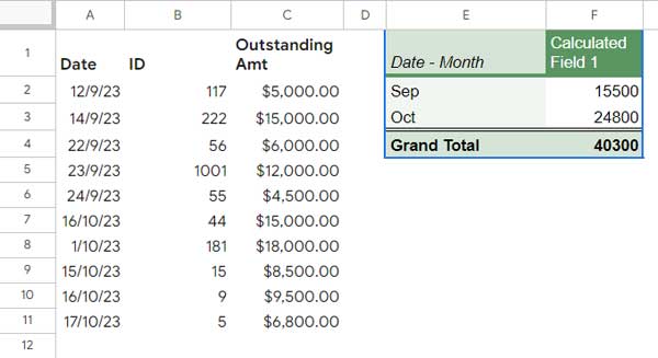
Example: SUMIF That Works in a Calculated Field
Consider a dataset with an Outstanding Amount field. If you want to sum values that are less than or equal to 10,000 within the same field, you can omit sum_range.
Working formula:
=SUMIF('Outstanding Amt', "<=10000")
✅ Why this works:
rangeandsum_rangeare effectively the same- No third argument is required
- Pivot table accepts the field label
Regular Pivot Table (Before Applying Condition)
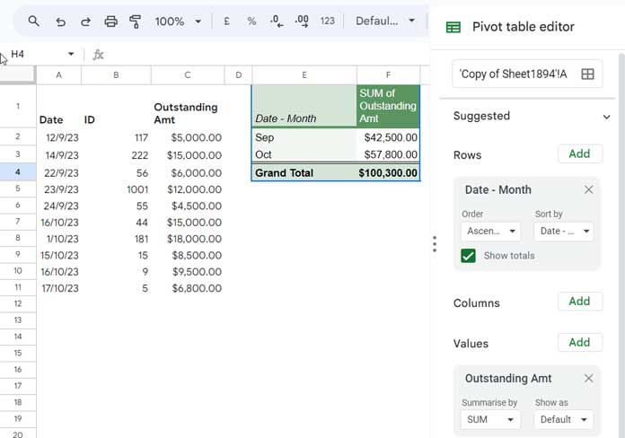
Before applying any conditions, here’s how the pivot table is set up.
The sample data is in the range A1:C, with dates in column A, product IDs in column B, and Outstanding Amount in column C.
In the pivot table:
- Date is added to Rows
- Outstanding Amt is added to Values
- The SUM function is used to summarize the values
After creating the pivot table, the dates are grouped by month by right-clicking on any date in the pivot table and selecting Create pivot date group → Month.
The resulting pivot table shows the total outstanding amount per month, as shown below.
👉 For a detailed walkthrough of creating and configuring pivot tables, see Google Sheets Pivot Table Basics & Setup.
Adding the Calculated Field

Conditional Sum Using SUMIF (Result)
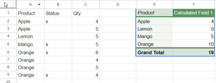
Example: SUMIF That Fails (Common Error)
Now consider a dataset with these fields:
- Product
- Status
- Qty
You want to sum Qty only when Status equals "x".
This formula looks correct, but fails:
=SUMIF('Status', "x", 'Qty')
❌ Returns: #N/A
(tooltip: “Argument must be a range”)
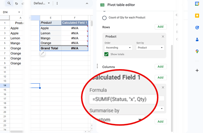
Why this fails
- Pivot tables do not treat
'Qty'as a valid range SUMIFrequiressum_rangeto be a true range reference- Field labels are not supported in this argument
This is one of the most common reasons users think calculated fields are “broken.”
Recommended Alternatives to SUMIF in Calculated Fields
Because SUMIF breaks when multiple fields are involved, the safest approach is to use functions that fully support pivot field labels.
Option 1: SUMPRODUCT (Recommended)
=SUMPRODUCT(Status="x",Qty)
✅ SUMPRODUCT Works reliably in calculated fields
✅ Cleaner syntax
✅ Best replacement for SUMIF in pivot tables
Option 2: SUM + FILTER
=SUM(IFNA(FILTER(Qty,Status="x")))
✅ FILTER + SUM Works correctly
⚠ Slightly more verbose than SUMPRODUCT
When You Don’t Need a Calculated Field at All
In some scenarios, a calculated field isn’t necessary.
For example, if you only need to include rows where Status = "x":
- Use Pivot Table Filters
- Exclude unwanted values directly in the pivot editor
However, calculated fields are still useful when you want:
- All categories displayed (including zero totals)
- Custom logic beyond simple filtering
- Reusable formulas that update automatically
Choosing the Right Approach
| Scenario | Best Approach |
|---|---|
| Same field condition | SUMIF (without sum_range) |
| Cross-field condition | SUMPRODUCT |
| Complex logic | SUM + FILTER |
| Simple inclusion/exclusion | Pivot table Filters |
Conclusion and Key Takeaways
SUMIF can be used in pivot table calculated fields in Google Sheets, but only in limited scenarios.
If your formula requires a sum_range, it will fail due to how pivot tables handle field references. In those cases, SUMPRODUCT is the most reliable and flexible alternative, followed by SUM + FILTER.
Key takeaways:
- Use
SUMIFonly whensum_rangeis not needed - Expect a #N/A error when SUMIF references multiple fields in a pivot table calculated field.
- Prefer
SUMPRODUCTfor conditional sums in calculated fields - Use pivot table filters when formulas are unnecessary
To learn more advanced pivot table techniques, explore other tutorials in the Pivot Table Calculations & Advanced Metrics in Google Sheets hub.


