In Google Sheets Pivot Tables, empty cells appear when a row–column combination has no corresponding record in the source data.

Unlike Microsoft Excel, Google Sheets currently does not provide an option to automatically display 0 for empty cells in Pivot Tables.

Even using a calculated field inside the Pivot Table editor cannot replace blank cells with 0.

However, there is a reliable workaround. By generating the missing records using a formula and adding them to the source data, the Pivot Table will automatically display 0 instead of blank cells.

This tutorial explains how to implement that workaround step-by-step.

This article is part of the hub “Pivot Table Formatting, Output & Special Behavior in Google Sheets.“

Why Pivot Tables Show Blank Cells Instead of 0

Before applying the workaround, it helps to understand the reason behind blank cells.

In a Pivot Table:

• Blank cell → No record exists in the source data
• 0 value → A record exists but the value is zero

For example:

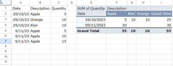
In this dataset:

• There are no records for Orange or Kiwi on 09-11-2023
• Therefore, the Pivot Table shows blank cells, not zero.

If a row existed with Quantity = 0, the Pivot Table would display 0 automatically.

Because of this behavior, automatically converting blanks to 0 could sometimes be misleading when analyzing data.

Still, many users prefer the Excel-style option to display 0 instead of blanks, which Google Sheets does not currently provide.

Until such a feature is introduced, the workaround below can help.

Step-by-Step Guide to Filling Empty Cells with 0 in Google Sheets Pivot Tables

Assume the source data is in A1:C, and the Pivot Table is placed next to it.

Create the Pivot Table

1. Select A1:C
2. Click Insert → Pivot table
3. Choose Existing sheet
4. Enter E1 as the destination
5. Click Create

Configure the Pivot Table as follows:

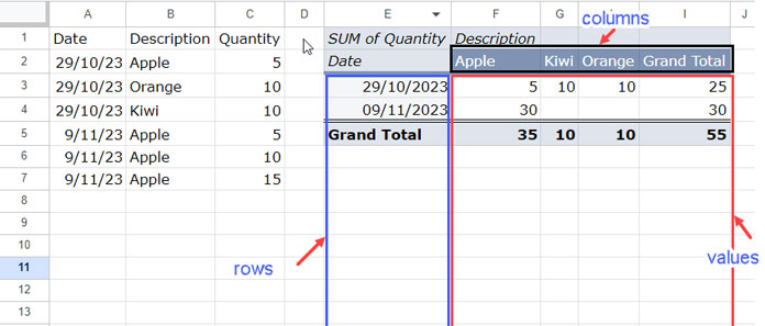
Rows

• Date

Columns

• Description

Values

• Quantity

Filter

• Date → Filter by condition → Is not empty

Your Pivot Table is now ready.

You will notice that some cells remain blank where records do not exist.

To convert these blanks into 0, we need to identify the missing row-column combinations.

Formula to Identify Missing Records in the Pivot Table

Instead of scanning the original data, we can use the Pivot Table output to detect missing combinations.

In the Pivot Table:

• Rows range → E3:E
• Columns range → F2:I2
• Values range → F3:I

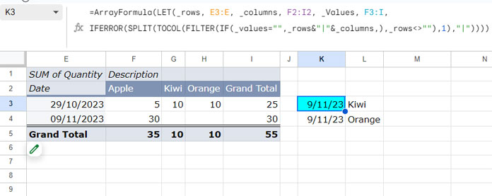
The following formula generates the missing records.

=ArrayFormula(
  LET(
    _rows, E3:E, 
    _columns, F2:I2, 
    _Values, F3:I, 
    IFERROR(SPLIT(TOCOL(FILTER(IF(_values="", _rows&"|"&_columns,), _rows<>""), 1), "|"))
  )
)

Important Notes

Date formatting

If the row labels are dates, format the output column:

Format → Number → Date

Adjusting for additional categories

If new categories are added to the source data, the Pivot Table will expand horizontally.

You must then adjust the ranges in the formula.

Example:

Original	After adding one more column
F2:I2	F2:J2
F3:I	F3:J

How the Formula Works

ArrayFormula

Allows the formula to return multiple rows of results automatically.

LET

The LET function defines variables inside the formula.

_rows → E3:E
_columns → F2:I2
_values → F3:I

This improves readability and performance.

IF Function

IF(_values="", _rows&"|"&_columns,)

If a Pivot Table cell is blank, the formula combines:

Date | Fruit

This creates the missing record identifier.

FILTER

FILTER(...,_rows<>"")

Removes extra rows below the Pivot Table.

TOCOL

Converts the results into a single column and removes empty cells.

SPLIT

Separates the combined values into two columns:

Date | Fruit

These are the missing records.

Final Step: Fill Empty Pivot Table Cells with 0

The Pivot Table was created using the open range A:C.

Now follow these steps:

1. Copy the formula results.
2. Scroll below your source data.
3. Leave a few blank rows.
4. Paste the results as values.

Match the columns exactly:

To paste values:

Right-click → Paste special → Paste values only

What Happens After Adding the Missing Records

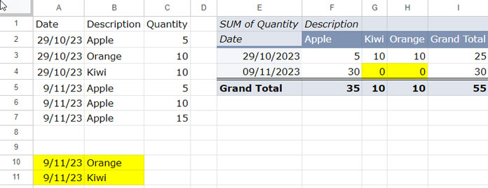
After adding the generated records:

• The Pivot Table now contains entries for every Date–Fruit combination
• Since the Quantity column is empty, the Pivot Table aggregation returns 0
• Previously blank cells now display 0

At the same time:

• The formula output becomes blank, since the missing records now exist.

If you are creating pivot-style reports using the QUERY PIVOT clause instead of the Pivot Table tool, see this guide: Replace Blank Cells with 0 in Query Pivot in Google Sheets.

Conclusion

Google Sheets does not currently provide a built-in option to fill empty Pivot Table cells with 0.

However, by detecting missing row-column combinations and adding them to the source data, you can force the Pivot Table to display zeros instead of blanks.

This workaround is especially useful when creating complete Pivot Table reports where every category must appear for every date or dimension.

For practice, you can use the sample sheet provided below, which contains two Pivot Tables. Follow the steps in this guide to generate the missing records and update the Pivot Tables.

Sample Sheet

More Google Sheets Pivot Table Tutorials

• Google Sheets Pivot Table Tutorial: Basics, Setup, and Date Grouping
• Pivot Table Calculations & Advanced Metrics in Google Sheets