Consolidate Data from Multiple Sheets Using a Formula in Google Sheets

Many people think there is no Excel Data Consolidation alternative in Google Sheets. Of course, there is no such command. But you can consolidate data from multiple Sheets using a formula in Google Sheets.

Don’t write off Google Sheets! There is a powerful function in Google Sheets to do data consolidation in a much better way! Do you know which function/formula is that?

I’m talking about the Query function. In this function, you can specify the data range in multiple Sheets in two ways.

Manual Entry (Hardcoded):- Use it when you have fewer Sheets to combine.

Using a Custom Named Function:- Use it when you have several Sheets to combine.

I’m using only the native functions, not Apps Script, or any third-party plugins, to consolidate data from multiple Sheets.

The data consolidation in this way is not limited to Sheets in a single file. You can use Sheets from even different files by importing them.

Understanding Consolidate Data from Multiple Sheets

I will combine data from multiple Sheets (multiple tabs in a workbook or file) into one single Sheet and then summarise it.

What about consolidating data in two workbooks in Google Sheets?

If that is the cause, you require to use the IMPORTRANGE function to import data first into a master Sheet.

I’ll skip that part in this tutorial to avoid unnecessary confusion.

Advantages of Using a Formula (Query Function)

Here are some of the advantages of consolidating data from multiple Sheets using a formula in Google Sheets

Data consolidation without any Script means better Spreadsheet performance.
Formulas are faster and more reliable if we write them correctly.
If we use any plugin (I don’t know about any such plugin at the time of writing this post), we can’t ensure the availability of that plugin always. Even if you find one, add it after reading the user reviews.
No need to pay any bucks to hire a developer to code an Apps Script for you.
When using a formula to consolidate data, you get more flexibility. The consolidated data will automatically get updated when we change the source data.

How to Consolidate Data from Multiple Sheets Using a Formula in Google Sheets

Please follow the step-by-step instructions below.

Below you can see four sheets (screenshots). The first two sheets, I mean sheet tabs, contain sample data which we will combine in the third sheet and summarise in the fourth sheet.

We can combine and summarise the data using one single formula. But to make the steps simpler, I am doing it separately.

Note:- You will get the detail to combine and summarise data using a single Query in the last part of this tutorial.

So there are two steps involved – data consolidation and combination. The third and fourth sheets we can use for this. I will split the tutorial below accordingly.

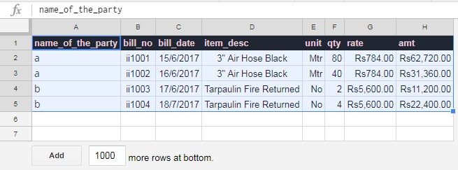
The first two sheets contain some sample data. See that below.

The name of my first sheet is junesheet, and here is the data in it.

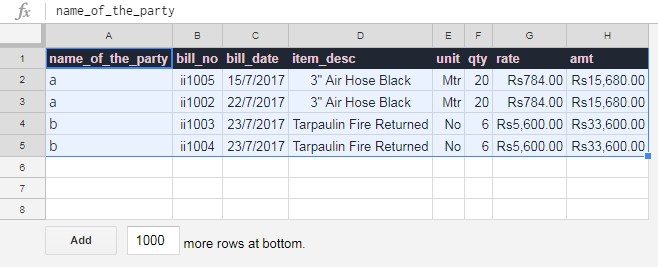
Now see the data in the second sheet named julysheet.

You can open my sample file below to see my data and formulas.

Data Consolidation Sample

How to Combine Data from Multiple Sheets Using Query Formula in Google Doc Sheets

Now let us see how to combine the above two sheets into a single sheet in the same Google Sheets file. I mean in the third sheet named Combined.

Below is the Query formula to combine the above two Sheets’ data into a single sheet.

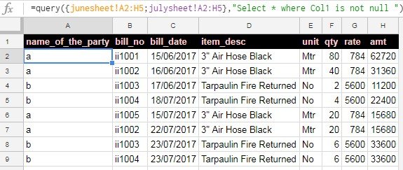
=query({junesheet!A2:H5;julysheet!A2:H5},"Select * where Col1 is not null ")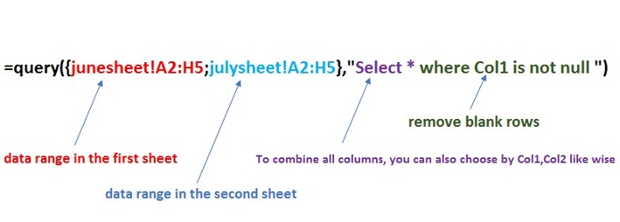

Consolidate Data from Multiple Sheets: Combining Data

The formula is for our sample data above. You can use it as it is but with changes suitable for your spreadsheet data. The changes that you may require to make may be as follows.

Change the range A2:H5 to your actual data range.
Change the sheet names to your actual sheet names.
I’ve used two Sheets to combine. Suppose there is one more Sheet to include named augsheet. Just put a semi-column and enter the third sheet name with the range.

E.g:-

{junesheet!A2:H5;julysheet!A2:H5;augsheet!A2:H5}

Important:- Combine only similar data types (avoid mixed data types in a single column). Never combine a text column with a date column or numeric column.

In your workbook, if column A contains text strings in the first sheet and numbers in the second sheet, don’t combine them. They will make the combined data mixed data type.

It’s against data consolidation using Query. The Query will return incorrect output when mixed data types are in columns.

Infinite Range in Consolidation

If you want you can use infinite ranges like A2:H in the formula. Then the formula will be like this.

=query({junesheet!A2:H;julysheet!A2:H},"Select * where Col1 is not null ")

Do you have several Sheets to combine? Then you may try one of these custom-named functions.

REF_SHEET_TABS: Reference a List of Tab Names in Query in Google Sheets.
COPY_TO_MASTER_SHEET: Combine Data in Multiple Tabs in Google Sheets.

We want to summarize or consolidate the data we combined from multiple Sheets. Below are the steps. Before that, first, see the combined data below.

Summarising or Consolidating Data from Multiple Sheets Using Query Formula in Google Sheets

The below part uses the Query function. You can also do this by using the Pivot Table.

Just by using one more Query formula in the last Sheet named “Consolidate,” we can achieve the required result.

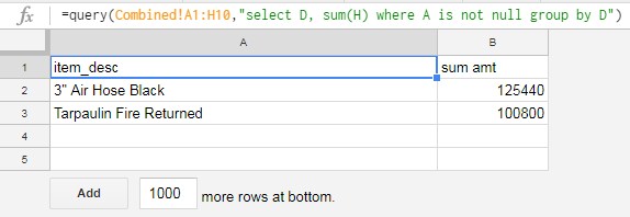
=query(Combined!A1:H10,"select D, sum(H) where A is not null group by D")

See this formula explained with the help of an image below.

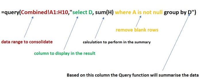
Consolidate Data from Multiple Sheets: Query Formula Explanation

I have used the Query grouping to perform Sum aggregation in this data consolidation formula.

In our sample data, column D contains the item description. I have summarised the data based on this item field.

When the same item appears multiple times, this formula merges that into one row and sums its values in column H.

The consolidated data will look as below.

Consolidate Data from Multiple Sheets Using Formula - Result Sheet

That’s all. I hope you enjoyed my tutorial and learned how to consolidate data from multiple sheets using a formula in Google Sheets.

As I promised at the beginning, here is the single formula that combines and summarises the data.

=query({junesheet!A2:H;julysheet!A2:H},"select Col4, sum(Col8) where Col1 is not null group by Col4")

What to Do if the Number of Columns is Different in Each Tab?

Usually, it won’t happen. But by any chance, if the number of columns in the data range in each tab is different, the above method doesn’t work.

You can try the below formula to first combine the data and then consolidate it.

Google Sheets: Combine Two Tables with Different Numbers of Columns in a Query.

The Query function is quite handy if you utilize it properly. So take your own time and learn the above Query function tutorial.

First, I thought about sharing some more Query tutorials here.

But there are 100+ Query tutorials on Info Inspired. So, better please use the Search bar to find it.

67 COMMENTS

Adam January 28, 2022 At 11:50 pm

Thank you for this tutorial. Is there a way to reference a dynamic set of tab names without changing the query formula?

For example, if I have the tab names in cells A1-A3, could I use ArrayFormula and Concatenate to put text in cell A4 that mirrors your reference range perfectly?

But I can’t seem to get the query to recognize that text as a valid set of references using the “INDIRECT(A4)” formula. Thank you.

- Prashanth January 31, 2022 At 10:56 am
  
  Hi, Adam,
  
  As far as I know, at present, the INDIRECT function is not capable of populating values from multiple tabs.
  
  You may find this tutorial useful – How to Include Future Sheets in Formulas in Sheets.
  
Yuvan September 2, 2021 At 4:21 pm

Hi, can you give the formula to combine data from 2 different files?

- Prashanth September 3, 2021 At 9:06 am
  
  Hi, Yuvan,
  
  Sure! I’ll update you soon.
  
Tessa Beach July 6, 2021 At 12:26 am

When I name my combined sheet a date range 7.1-7.4? It messes up the query. How do I fix it?

- Prashanth July 7, 2021 At 2:16 pm
  
  Hi, Tessa Beach,
  
  Enclose the tab names within single quotes.
  
  E.g.:-
  
  =query({'7.1-7.4'!A2:H5;'7.5-7.10'!A2:H5},"Select * where Col1 is not null ")
  
beibei May 25, 2021 At 8:37 am

Hello! Do you have tutorial for consolidating multiple spreadsheet from different files? Thank you

- Prashanth May 25, 2021 At 9:33 am
  
  Hi, beibei,
  
  You can combine multiple Spreadsheet files dynamically in Google sheets by following my below tutorial.
  
  How to Combine Multiple Sheets in Importrange and Control Via Drop-Down.
  
  For summarize, then you can use QUERY – IMPORTRANGE.
  
Nana October 27, 2020 At 9:55 am

Hello, I’ve been doing this for quite a while but I just started a new sheet and instead of adding the combined in one column, it expanded to other columns on the right, I used the exact same coding as you did here.

- Prashanth October 28, 2020 At 11:36 am
  
  Hi, Nana,
  
  The new sheet may have different Locale settings. You can check that from the menu File > Spreadsheet settings from within that sheet.
  
  To read more about the locale setting and its impact on the result, please check my corresponding tutorial. The link already shared above (within my reply to Sarah).
  
Michelle Frisone September 26, 2020 At 6:03 am

Hi,

I am trying to make a master schedule from different schedules all in the same google sheet file. I tried using your formula and am getting the following error:#ERROR! Formula parse error.

I am trying to show a full schedule in a master sheet so I can see who’s doing what and when. The data is all text, not mixed. What am I doing wrong? It also failed when I tried to do it using the ARRAY as well.

Thank you!

- Prashanth September 29, 2020 At 9:12 am
  
  Hi, Michelle Frisone,
  
  I could not see a sheet with your expected result within your shared file. Please add one more tab showing your expected result and share the sheet link again.
  
Rafael Miranda September 22, 2020 At 11:21 pm

The formula isn’t working for me. Could anyone please help me identify what is wrong?

– link removed by admin –

- Prashanth September 23, 2020 At 11:13 am
  
  Hi, Rafael Miranda,
  
  Here is the formula that I could find on your sheet named “Query”
  
  =QUERY({'Only Departures'!A2:L;'Only Arrivals'!A2:L};"SELECT *")
  
  It’s actually correct. But in the above consolidation formula, you have used two open ranges, i.e A2:L. So between two tables, there are several blank rows, that is why you can’t see the second table (“Only Arrivals”) below the first table (“Only Departures”).
  
  To see that, use the below Query consolidation formula.
  
  =QUERY({'Only Departures'!A2:L20;'Only Arrivals'!A2:L20};"SELECT *")
  
  But the ideal way to solve this problem is to include the WHERE clause in Query as below.
  
  =QUERY({'Only Departures'!A2:L;'Only Arrivals'!A2:L};"Select * where Col2 is not null";0)
  
  You can learn more about all the Query CLAUSES here – What is the Correct Clause Order in Google Sheets Query?
  
  - Rafael Miranda September 23, 2020 At 5:10 pm
    
    Hats off for you, brother. Thanks a lot!
    
Zyshan September 10, 2020 At 2:22 pm

Can please guide me over this issue.

=QUERY({Cash!A2:T10000;Online!A2:T10000}, "Select G, H, I where H = '"&$A2&"' and G > date '"&TEXT(D1,"yyyy-mm-dd")&"' and G <= date '"&TEXT(E1,"yyyy-mm-dd")&"'")

- Prashanth September 11, 2020 At 11:17 am
  
  Hi, Zyshan,
  
  Since you have used the expression {Cash!A2:T10000;Online!A2:T10000} as the ‘data’ in Query, you should use column identifiers as below.
  
  "Select Col7, Col8, Col9 where Col8="
  
  I hope you could change the formula accordingly.
  
Nicky Palmer June 11, 2020 At 10:09 pm

Hi, thank you so much for this, really helpful!

I’m having a problem with some data not being recognized as numbers and I can’t work out why! Please can you help?

This is my formula:

=QUERY({UK!A5:W; RU!A5:W; PT!A5:W; FR!A5:W; IT!A5:W; BE!A5:W; ES!A5:W; NL!A5:W; NO!A5:W; CH!A5:W; DE!A5:W; AT!A5:W; DK!A5:W; SE!A5:W; CA!A5:W; UAE!A5:W; AU!A5:W},"select * where Col1 is not null")

Thanks,

Nicky

- Prashanth June 12, 2020 At 10:33 am
  
  Hi, Nicky Palmer,
  
  I can solve if I can see the formula live (on a sample sheet).
  
  Please do avoid using mixed-type data columns in Query formulas (eg. a column that contains both numbers and texts) as Query may ignore some of the values from such columns.
  
Shikamu January 29, 2020 At 1:33 am

I’ve tried to play a bit more with the script editor and it looks like I’m able to do what I want there. It is, however, pretty slow 🙁

- Prashanth January 29, 2020 At 9:22 am
  
  Hi, Shikamu,
  
  Thanks for your update!
  
Shikamu January 26, 2020 At 4:28 pm

What if you have many many sheets like your ‘junesheet’ and ‘julysheet’, and you don’t want to have to type each of them? Is there a way to consider all sheets from a certain index or something?

- Prashanth January 27, 2020 At 9:21 am
  
  Hi, Shikamu,
  
  In Excel, there is a way to achieve that keeping the tab names as a list in a column and then using Indirect and Sumproduct. Unfortunately, it doesn’t work in Google Sheets.
  
  - Shikamu January 27, 2020 At 2:21 pm
    
    Hi, thanks for your answer!
    
    Do you have any idea how I could use my data then? Is there a “better” way for me to “format” it? so that I could then perform the queries I’m interested in. e.g. rather than making a sheet per day with the data, just have it all in one sheet? or one per month might already make it easier. But then working out where “each data set starts” will be a bit challenging and I’m guessing I won’t be able to do that dynamically either so back to square 1…
    
    - Prashanth January 27, 2020 At 3:45 pm
      
      Hi, Shikamu,
      
      It will be a very time taking and error-prone process to consolidate a bunch of sheets. As you have suggested, split your data month wise or use a single sheet.
      
      Can I see a mockup of the data that you are working with? So that I can possibly give you a better reply.
      
zain Kamze January 24, 2020 At 4:26 am

Hello,

I really appreciate ur efforts. I encountered one problem while combining different sheets(tabs) into one master sheet, e.g I have three sheets named “Cola”, “Pepsi” & “Thumbsup”.

I consolidated their results all in my Master sheet using Query formula with null.

Whenever anyone entered data in “Cola”, “Pepsi” & “Thumbsup” sheet, it comes to my master sheet somewhere between the rows. I need it to comes queue wise, is it possible?

The problem I faced is, I am writing a remark on my master sheet on each entry so whenever someone added new data in “Cola”, “Pepsi” & “Thumbsup”, it’s inserted in between the data and break the sequence of my remarks.

- Prashanth January 24, 2020 At 9:48 am
  
  Hi, zain Kamze,
  
  You need unique ID columns in each sheet (for example in column 1 in each sheet).
  
  In Column 1 in a master sheet, consolidate only the Unique ID columns from each sheet. In column 2 in the master sheet, you need to use a Vlookup in which the search keys will be column 1 values from the same sheet, the range will be the consolidated three tabs, and index numbers will be {1,2} etc. based on the number of columns to pull.
  
  A similar approach I have already detailed here.
  
  Align Imported Data with Manually Entered Data in Google Sheets
  
Külli January 14, 2020 At 4:34 pm

Hi, thanks for the great tutorial!

It saved my day(s)! Well, almost… as for some strange reason the formula does not put those sub tables under each other, but next to each other?!?!

=QUERY({Sheet1!A2:X,Sheet2!A2:X,Sheet3!A2:X,Sheet4!A2:X,Sheet5!A2:X},"Select * where Col1 is not null",0)

Could you please advise, what could be the problem?

Thank you already in advance!

- Külli January 14, 2020 At 4:46 pm
  
  Well, magically it all worked out when I replaced commas between subtables with semi-colons! 🙂 Thanks again! You are the best!
  
- Prashanth January 14, 2020 At 4:51 pm
  
  I wish I could see your sheet! Because ‘locale’ settings (File menu > Spreadseeht settings) can affect the result.
  
  At least share a sheet with mockup data. So that I can help you solve the said Query formula issue.
  
Joseph December 11, 2019 At 2:01 am

Hi, great tutorial, thank you very much! I have an issue though :/

I use this formula : QUERY({zorro;vador};”select *”). “zorro” and “vador” are named ranges in 2 different sheets. The problem is that the header gets repeated.

- Prashanth December 11, 2019 At 1:49 pm
  
  Exclude the header row (by modifying the named range) from one of the named ranges.
  
Adi December 2, 2019 At 7:44 pm

Hi Prashanth,

Please write an article on consolidating data from multiple sheets from multiple files!

I am trying to make a CRM that works with Google Forms responses. For example, I have the main sheet with Name, Email, and Phone, and I have a form that has Name, Email, and Budget. I want to combine them in the same sheet and same row. I also plan to expand and use more forms with this structure.

TIA!

- Prashanth December 2, 2019 At 8:51 pm
  
  Hi, Adi,
  
  Please go thru’ this tutorial.
  
  How to Vlookup Importrange in Google Sheets [Formula Examples]
  
  If this is not what you are looking for, please make two sample sheets and share them here.
  
  Let’s try.
  
  Best,
  
Heather Martins November 20, 2019 At 6:30 pm

This is my formula.

=query({Issue Log!A2:AP;Issue Log Archive!A2:AP},"Select * where Col5 is not null ")

I get a formula parse error.

Both sources are from Import ranges.

- Heather Martins November 20, 2019 At 6:42 pm
  
  I figured it out. I changed it to;
  
  =query({'Issue Log'!A2:AP;'Issue Log Archive'!A2:AP},"Select * where Col5 is not null") and it worked.
  
david October 15, 2019 At 11:06 pm

Hello Prashanth,

This is a great way to learn. I am a great follower of your site. Thank you for sharing your work.

I am using the following Query formula to consolidate data from multiple sheets. However, if I try to take out some results using NOT Col3 contains 'Lorem ipsum', the results are eliminated but replaced by the cell value in other Sheet since this value is repeated several times.

How can I completely eliminate the query results even if the value is repeated in several sheets?

=SORT(SORTN(QUERY({Entrada_OFI!A2:D; Salida_MA!A2:D; Entrada_MA!A2:D; Salida_a_Proyecto!A2:D}; "Select Col4, Col3, Col2, Col1 where UPPER(Col4) contains UPPER('"&B3&"') and NOT Col3 contains 'Salida a Proyecto' order by Col1 desc");9^9;2;3;TRUE); 2; 0)

- Prashanth October 16, 2019 At 9:00 am
  
  Hi, David,
  
  I have tested the formula in a demo sheet and it works fine for me. It consolidates the data and filters the column 4 for the values match the criterion in cell B3 and column 3 not equal to ‘Salida a Proyecto’.
  
  Can you explain what you meant by saying “The results are eliminated but replaced by the cell value in other Sheet since this value is repeated several times”?
  
  Best,
  
Mohammed Ashraf August 26, 2019 At 10:38 am

Thanks a lot.

Japoy August 23, 2019 At 7:04 am

Hi @Prashanth,

I’m having a bit of a problem. Hope that you can help me.

I used an Importrange to import different spreadsheets into one sheet then used the {;} formula and the Query to consolidate it into one sheet.

It worked fine but when I put 3 to 4 sheets, one of the columns disappears. I am really in peril right now. Hope you can help me. Thanks.

- Prashanth August 23, 2019 At 8:22 am
  
  Hi, Japoy,
  
  Can you replicate the error with some sample data and share? I am confident that I can help you then.
  
  - Japoy August 23, 2019 At 9:15 am
    
    Hello Prashanth,
    
    Thank you for responding. I can. Would you let me know your email so I can send you a sample file? Thanks.
    
    - Prashanth August 23, 2019 At 5:25 pm
      
      Hi, Japoy,
      
      You can share the link via comment itself. I won’t publish the link. Even if I publish, it would be a copy of the same from my drive.
      
      Best,
      
a August 15, 2019 At 3:56 pm

Hi. How about if I want to consolidate sheet from 2 files?

- Prashanth August 16, 2019 At 10:24 am
  
  Hi,
  
  Use the Importrange function to import the data and then consolidate it.
  
  Google Sheets Importrange Function – Basic to Advanced Use Tips
  
Lisa August 10, 2019 At 4:31 am

Is there a way to alphabetize the combined sheet?

- Prashanth August 10, 2019 At 1:23 pm
  
  Hi, Lisa,
  
  Yes, of course!
  
  =query({junesheet!A2:H5;julysheet!A2:H5},"Select * where Col1 is not null order by Col1 Asc")
  
  Best,
  
Sanjay July 3, 2019 At 5:02 pm

I have 5 sheets which have the data and each has a total column at the end of each sheet
I want to pull that total number row from each sheet to a master sheet
How can I do this can u pls guide me.

- Prashanth July 4, 2019 At 4:40 pm
  
  Hi, Sanjay,
  
  In the below post I have included the formula to consolidate the total row in two sheets. You can tune that for 5 or more sheets.
  
  Consolidate Only the Last Row in Multiple Sheets in Google Sheets
  
Nate June 23, 2019 At 5:30 am

This is exactly what I’ve been looking for! Thank you!

To take it a step further, is it possible for the data ranges to be referenced from a table?

The ranges I’m combining are the same cell range on different sheets, and I’d prefer that the user doesn’t have to update the formula when they add a new sheet.

I can only seem to get INDIRECT to work with one range. Any ideas?

- Prashanth June 23, 2019 At 8:48 am
  
  Hi, Nate,
  
  I know this problem prevails with the Indirect function in Google Sheets. It won’t work with array as you think.
  
  So, if you want you can think about this workaround.
  
  Assume, you want to combine 5 Sheets and your workbook only contain 4 sheets right now. See how I have included the fifth Sheet in the formula.
  
  The range to combine in each Sheet is A1:B4.
  
  =iferror(ArrayFormula({Sheet1!A1:B4;Sheet2!A1:B4;Sheet3!A1:B4;Sheet4!A1:B4;iferror(Sheet5!A1:B4,” “/COLUMN(A1:B1))}))
  
  This works if you can predict (predetermine) the future Sheet names.
  
  Best,
  
  Prashanth KV
  
Tish June 8, 2019 At 2:13 am

Wow, this is great. However, on the “Combined” sheet, is there a way to be able to filter or format the sheet? Is there any way to have a combined sheet that when edited updates the sheets feeding it?

TIA, Tisha

- Prashanth June 8, 2019 At 8:00 am
  
  Hi, Tisha,
  
  You can filter the data in the combined Sheet.
  
  This formula filters only the invoice no “ii1002′
  
  =query({junesheet!A2:H5;julysheet!A2:H5},"Select * where Col2='ii1002' ")
  
  You can’t edit the combined sheet and get the source (the data feeding it) get updated.
  
  Best,
  
Balaji January 3, 2019 At 8:36 am

Is it possible to add Sheet name in the combined list?

Sarah December 28, 2018 At 3:24 am

I’m trying to use the following formula to locate an employee name on the corresponding month tab, and then find the number of PTO hours used, and subtract them from the total available hours on a primary sheet.

Using the formula below, I am able to have it work correctly for January, but when I add the other months, nothing happens.

=40-SUM(QUERY({January!A:Q; February!A:Q; March!A:Q; April!A:Q},"select Col14 where Col1 = 'Brittney Albeck'"))

I’m thinking my problem is that I am attempting to combine a number that is found based on a texts location on the sheet, and that’s not coming across correctly in my formula.

Suggestions

- Prashanth December 28, 2018 At 12:31 pm
  
  Hi, Sarah,
  
  The formula would be something like this.
  
  =40-QUERY({January!A:Q; February!A:Q; March!A:Q; April!A:Q},"select sum(Col4) where Col1 = 'Brittney Albeck' label Sum(Col4)''")
  
  Please note that the values in column D in all the tabs must be numbers, not mixed data types.
  
  Further, if you are from any of the EU countries, you might want to change the semicolon in the formula.
  
  How to Change a Non-Regional Google Sheets Formula
  
  Hope this may help.
  
  Best,
  
John Kyle December 20, 2018 At 8:32 am

Thank you so much for this! I’m building my own spending/tracking budget GSheet to use instead of YNAB or Mint. I have a separate tab for each account and needed a way to see how much I’m spending in each category across the tabs. Your query works great to create a combined tab, and then I used a pivot table which references the combined tab to show the sum of spending from each month.

I couldn’t figure out how to filter by date using a query, so I just used the pivot table, but I have to use a hack to get all the categories to show up in the pivot tables, even if $0 for the month. I created a tab that shows all the categories with $0 and pulls this into the combined tab along with the accounts.

Cool stuff, thanks!

Amanda Moore December 15, 2018 At 10:11 pm

Is there a way to do this and Keep the cell color from the selected sheets?

- Prashanth December 17, 2018 At 9:30 am
  
  As far as I know, it’s not possible using traditional formulas. But I am unsure about add-ons.
  
Beppe Allegretta December 12, 2018 At 8:14 pm

Hi Praatek,

What about tables with different row numbers? I mean how to consolidate tables putting one below the other? Consider that row number may vary every day so.

Thanks in advance.
Beppe

- Prashanth December 13, 2018 At 8:52 am
  
  Hi, Beppe Allegretta,
  
  You can consolidate two or more tables with different row numbers.
  
  See my last Query formula (just above the Conclusion section) that handles infinite ranges like A2:H. But make sure that the number of columns are the same.
  
  Thanks.
  
Prateek Bansal December 1, 2018 At 11:19 am

Hey, thank you so much for this functionality. I have one query. I have added links to text and I want to move that as well when I combine two sheets. For example:- On text “Click Here” I have added a link abc.com but when I use the above example the link disappears. Can you help me in moving the link as well?

- Prashanth December 3, 2018 At 8:13 am
  
  Hi, Prateek Bansal,
  
  It’s not supported in Query function.
  
popun patro June 18, 2018 At 5:54 pm

When I use this formula value error shown and comment as “unable to parse query string for function QUERY parameter 2: NO_COLUMN:col1” please help.

- Prashanth June 18, 2018 At 9:22 pm
  
  Did you put that Curly Brackets?
  Please show me your formula.
  
Raj May 6, 2018 At 2:45 pm

Very Much Helpfull!! Thanks a lot

Arik March 25, 2018 At 3:44 am

That was very helpful! thanks!