Need to combine data from multiple sheets without editing your QUERY formula every time you add or remove a sheet?

This tutorial shows you how to query multiple sheets using a list of sheet names in Google Sheets. The solution lets you dynamically include or exclude sheets with checkboxes, supports future sheet names, and returns a combined array that you can use in any QUERY formula.

Quick Answer

Use the formula in this tutorial to:

• Combine data from multiple sheets listed in a column.
• Dynamically include or exclude sheets using checkboxes.
• Ignore sheet names that do not yet exist.
• Remove blank rows automatically.
• Pass the combined data directly to the QUERY function.

Why Use a List of Sheet Names in QUERY?

Maintaining a list of sheet names instead of hardcoding them inside a QUERY formula offers several advantages.

• No need to edit the formula whenever you want to include or exclude sheets.
• Future sheet names can already exist in your list without breaking the formula.
• Checkboxes let you dynamically select which sheets to include.
• The same combined data can be used in QUERY, FILTER, SORT, PIVOT, or other array-based formulas.

Before You Begin

To use this solution successfully:

• All source sheets must have the same column structure.
• Corresponding columns should contain the same type of data. For example, avoid combining a Date column with a Text column in the same position.
• Every sheet should have the same header row.
• Enter one sheet name per row in the tab list.

How to Query Multiple Sheets from a List of Sheet Names

You can follow this tutorial using the sample spreadsheet below.

Copy Sample Sheet

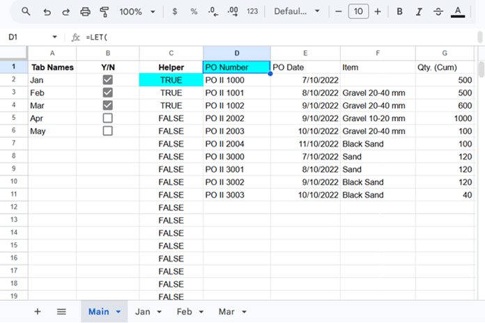
Assume your workbook contains three sheets named Jan, Feb, and Mar. Each sheet contains data in A1:D, where A1:D1 is the header row.

Create another sheet in the same workbook and enter the sheet names in column A, starting from A2.

You can also include future sheet names such as Apr and May.

Next, insert checkboxes in column B beside each sheet name.

To do that, select the required cells and choose:

Insert > Checkbox

Tick the checkboxes for the sheets that you want to include in the QUERY.

Step 1: Verify That the Sheet Names Exist

Enter the following formula in C2.

=MAP(
  A2:A,
  LAMBDA(r,
    AND(
      r<>"",
      IFERROR(SHEET(TO_TEXT(r)), 0)
    )
  )
)

This helper formula checks whether each sheet name actually exists in the workbook.

If you would like to learn more about this technique, see my tutorial on the SHEET and SHEETS functions.

Step 2: Combine the Selected Sheets

Enter the following formula in D1.

=LET(
  tabList, A2:A, 
  include, B2:B, 
  helper, C2:C, 
  dataRange, "A2:D", 
  header, INDIRECT(A2&"!A1:D1"), 
  fData, 
    REDUCE(
      header, 
      FILTER(tabList, include*helper), 
      LAMBDA(acc, val, 
        VSTACK(acc, LET(data, INDIRECT(val&"!"&dataRange), FILTER(data, CHOOSECOLS(data, 1)<>"")))
      )
    ), QUERY(fData, "select *", 1)
)

Customize the Formula

You only need to modify these parts.

Using Your Own QUERY

The formula currently returns all rows.

Replace this section:

QUERY(fData, "select *", 1)

with your own QUERY statement.

For example:

QUERY(fData, "select Col3, sum(Col4) group by Col3", 1)

You can use any valid QUERY expression because fData already contains the combined data from all selected sheets.

How the Formula Works

The formula combines multiple sheets in three stages.

FILTER selects the required sheets

FILTER(tabList, include*helper)

This returns only the sheet names that:

• are checked, and
• actually exist in the workbook.

REDUCE processes each sheet

The REDUCE function loops through every selected sheet name.

For each sheet, it:

• builds the sheet reference with INDIRECT,
• retrieves the specified data range,
• removes blank rows,
• appends the data underneath the previous sheet using VSTACK.

QUERY analyzes the combined data

After REDUCE finishes, all selected sheets become one continuous array.

The QUERY function then performs filtering, aggregation, grouping, sorting, or pivoting on that combined dataset.

Troubleshooting

QUERY returns unexpected results

Make sure every source sheet has the same layout.

For example, if column B contains dates in one sheet, it should not contain text in another.

Blank rows appear

The formula removes blank rows based on the first column.

If your first column can legitimately contain blank values, modify the FILTER condition to use another column.

No data is returned

Check that:

• at least one checkbox is selected,
• the selected sheets contain data,
• the specified data range is correct.

Frequently Asked Questions

Can I add future sheet names?

Yes.

You can list future sheet names in column A before creating those sheets. The helper formula prevents non-existent sheets from being included.

Can I include or exclude sheets without editing the formula?

Yes.

Simply tick or untick the corresponding checkbox.

Can I use this combined data in formulas other than QUERY?

Yes.

You can replace QUERY with FILTER, SORT, UNIQUE, or any function that accepts an array.

Does this work with hidden sheets?

Yes.

As long as the sheet exists and its name appears in the list, it can be included.

Conclusion

Using a list of sheet names makes it much easier to manage a QUERY that combines data from multiple sheets. Instead of editing the formula whenever you add, remove, or temporarily exclude a sheet, simply update the list or toggle the corresponding checkbox.

Because the formula returns a standard array, you can use it not only with QUERY but also with many other Google Sheets functions that work with dynamic arrays.