In this walkthrough guide, you can learn how to create, use, edit, delete, and import named functions in Google Sheets.

What more! You will find a growing list of named functions at the end of this post.

During 2022-2023, Google Sheets got new functions, features, and a UI overhaul. I like most of the new features available in my account, except the Data Validation. As a side note, I don’t have the new Timeline in my account. Since I used MS Project and

Let’s focus on Named functions. It’s also a new feature added to Google Sheets to help users to create custom functions without the help of Google Apps Script.

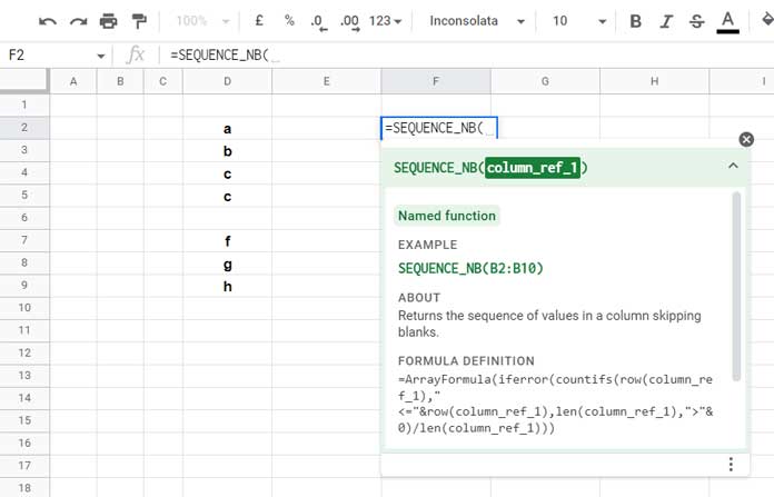
For example, we can create a custom function named SEQUENCE_NB to number a column in Sheets.

Unlike the built-in SEQUENCE, this newly created function will number only in rows where the referred column has any value.

Function Tip as you Type:

Formula Output:

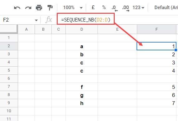
We can reuse this function similarly to any built-in function in Google Sheets like =SEQUENCE_NB(A2:A), =SEQUENCE_NB(Sheet2!I:I), etc. Further, Google Sheets supports importing this function into other Sheets.

When should you consider creating a named function in Google Sheets?

In short, use this feature when you have a complex Google Sheets formula in hand and want to reuse it in the same or different workbooks more often.

Custom Functions Using Built-in Formulas in Excel and Sheets

Excel:

Excel for Microsoft 365 already has a similar feature where we first convert our formula to a LAMBDA and then copy-paste that within Name Manager to create a Named Function.

Google Sheets:

In Google Sheets, we don’t want to write the LAMBDA first.

We can directly copy-paste the formula within Named functions (Data > Named Functions [Under the Data menu]).

From within that interface (a sidebar panel), we should replace cell/range references in the formula with placeholders (text) for inputs.

For example, you can replace A2:A in the formula with meaningful text like column_reference.

That’s the difference between creating custom functions in Excel and Google Sheets.

The Role of LAMBDA

Then why should we have the LAMBDA function in Google Sheets?

It has a few associated helper functions (LHFs), and that can make a killer combination.

Further, we can use the LHFs to create a named function in Google Sheets. We will discuss that in a later tutorial.

How to Create a Named Function in Google Sheets

Below we are going to convert two useful formulas into named functions.

SEQUENCE_NB (One Argument)

First and foremost, we require a working formula to create a named function in Google Sheets.

Let’s start with a formula that skips blank rows in sequential numbering.

You can find a number of formulas for this type of numbering in Google Sheets, and here is one.

=ArrayFormula(if(len(B2:B9),countifs(row(B2:B9),"<="&row(B2:B9),len(B2:B9),">0"),""))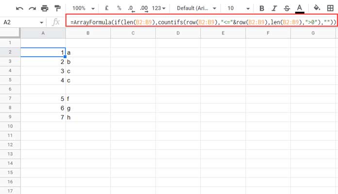

In this Google Sheets formula, we have one unique range reference and that is B2:B9. So the custom function may only require one argument (placeholder).

Steps

1. Copy the above formula.
2. Go to Data > Named functions > Add new function.
3. Enter the function name, i.e., SEQUENCE_NB. When defining a function name, you should avoid using the following types.
   • Any built-in function name in Sheets.
   • TRUE or FALSE Boolean values.
   • A1 or R1C1 syntax.
   • Spaces and Special characters except for the underscore.
   • Name starting with a number.
   • Longer names, i.e., above 255 characters
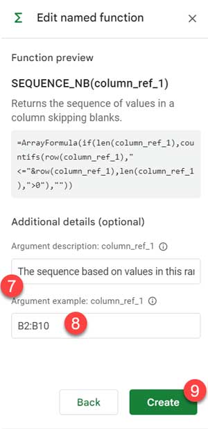
4. A meaningful description of the function. Here input “Returns the sequence of values in a column skipping blanks.“
5. Under argument placeholders, enter the argument name, i.e., column_ref_1.
   • For e.g., if you check the built-in MAX function syntax which is MAX(value1, [value2, …]), the argument placeholders are value1 and value2.
   • Here also, bullet points 3, 4, and 5 under the third point above are specifically applicable.
6. Under the formula definition, paste the earlier copied formula and edit it to replace B2:B9 with the placeholder column_ref1. Then it will be as follows: =ArrayFormula(if(len(column_ref_1),countifs(row(column_ref_1),"<="&row(column_ref_1),len(column_ref_1),">0"),""))
7. Click the “Next” button and fill in additional details for the placeholder name (column_ref_1). I have put “The sequence based on values in this range.“
8. Finally, put the argument (colum_ref_1) example. Here I have put B2:B10.
9. Click the “Create” button.

Adding a New Function # 1:

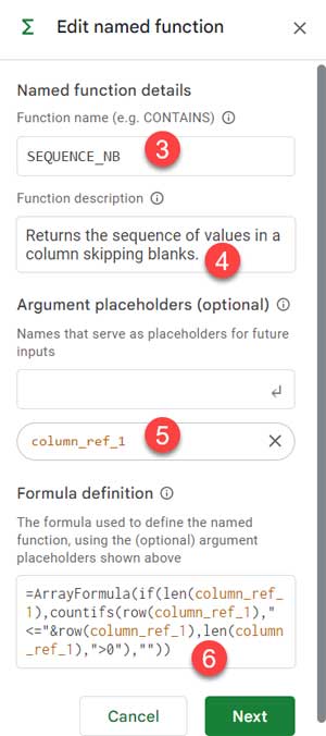
Adding New Function # 2:

You have created your first named function in Google Sheets.

Now you can use this function similar to any other built-in function from within any sheet in that workbook.

FLIP_DATA (Two Arguments)

In this example, let’s create a named function called FLIP_DATA.

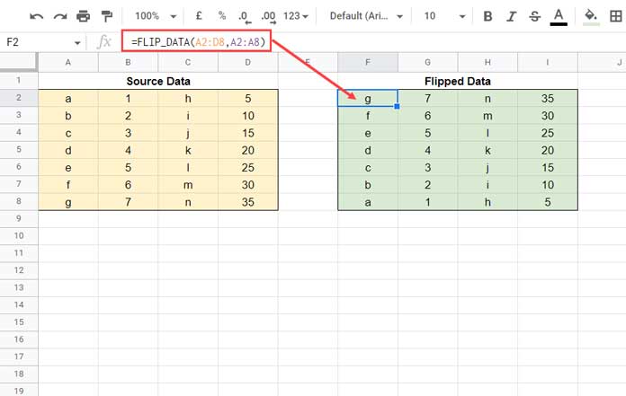
As the name suggests, we can then use this function to flip a data range in Google Sheets.

The following formula will flip the range A2:C5.

=SORT(A2:C5,ROW(A2:A5)*N(A2:A5<>""),0)

There are two unique range references in this formula.

So we may require two arguments (placeholders) in the custom FLIP_DATA function, and here are they – flip_range and first_col_range.

Steps

1. Copy the above formula.
2. Go to Data > Named functions > Add new function.
3. Enter the function name, i.e., FLIP_DATA.
4. Enter a meaningful description of the function. Here input “Provided a range, the function returns a vertically flipped data.“
5. Under the argument placeholder, add argument names, i.e., flip_range and first_col_range.
6. Under the formula definition, paste the earlier copied formula and edit it as follows – =SORT(flip_range,ROW(first_col_range)*N(first_col_range<>""),0).
7. Click the “Next” button and fill in additional details for the placeholder name. For flip_range, put “The data range to flip vertically,” and for first_col_range, key in “The first column reference in the data range to flip.“
8. Finally, put arguments examples. Here I have keyed in A2:C5 and A2:A5, respectively.
9. Click the “Create” button.

We can use the above-created named function to flip data in a single or multiple columns range.

How to Delete or Modify Named Functions in Google Sheets

To delete or modify named functions, go to Data > Named functions.

You can see all your custom functions in that.

Click the vertical three dots against a function and choose either “Edit” or “Remove.”

It’s that simple!

Please note that there is no option to delete multiple named functions in one go.

Importing Named Functions from One Workbook to Another

Create all your required named functions in a sheet and later import them to other sheets.

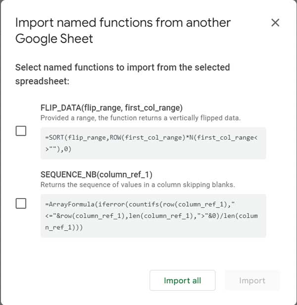
Assume you have the above two custom functions in the file “Google Sheets Named Functions.” You can keep this file opened or closed.

Let’s see how to import these two named functions into another workbook.

1. Open a new Google Sheet file.
2. Go to Data > Named functions.
3. Click Import function
4. Select the file in which you have created the two named functions.
5. Click Import All or select the function that you want to import, and voila!

This way we can create and reuse named functions in Google Sheets.

Get My Named Functions Created in Google Sheets

1. PUNCH_IN_OUT_SAME_ROW: To Copy Punch Out Time to the Punch In Row.
2. COPY_TO_MASTER_SHEET: Combines Data in Multiple Tabs in Google Sheets.
3. MERGE_TABLE_REMOVE_DUPLICATES: Removing Duplicates by Key Column.
4. COMPARE_ALL_COLUMNS: Compares All Columns with Each Other for Duplicates.
5. NEXT_RENEWAL_DATE: Get the Next Renewal Date (Monthly and Yearly).
6. AGE_CALC: To Calculate Age or Duration.
7. REPT_ROWS: Repeats Each Row in a Table by Varying N.
8. GANTT_CHART: An Easy Way to Create Gantt Charts.
9. LIST_ALL_DATES: Populates Dates Between Two or More Given Dates.
10. AT_EACH_CHANGE: Aggregation Results at Value Change Rows.
11. CUSUM_BY_GROUP: Running Total by Group (Item, Month, or Year).
12. SPARKLINE_NEGATIVE_BAR: SPARKLINE for Positive and Negative Bar Graph (Array Formula).
13. REF_SHEET_TABS: Reference a List of Tab Names in Query in Google Sheets
14. _3D: Creates a 3-D reference in Google Sheets.
15. SPLIT_EXPENSES: Splits group expenses.
16. NUMBERTOWORDS: Converts numbers to words in Google Sheets.
17. CUSTOMTIMESLOTS (new!): Creates custom time slot sequences.
18. TOSENTENCECASE (new!): Converts a specified string to sentence case.

Thanks for the stay. Enjoy!