As of the writing of this tutorial, a 3-D reference is not supported in Google Sheets. You may need a third-party add-on or a workaround formula to achieve this.

We will use the REDUCE Lambda function to code a formula and a custom function to make 3-D referencing possible in Google Sheets.

“A 3-D reference is most useful when you work with a Google Sheets file that contains several sheets of similar types of data. For example, account statements such as outstanding liabilities of different cost centers

So when you want to total the liabilities, you may want to use a 3-D reference like =SUM(Sheet1:Sheet5!C10). But it won’t work in Google Sheets. We require to adopt a workaround as mentioned above.

But don’t expect the flexibility you may get in Excel with our workaround formula in Google Sheets. For example, you may have to compromise when naming sheets.

I mean, you should follow a naming pattern when you name your sheets (tabs). For example, you could use “Sheet1”, “Sheet2”, “Sheet3”, or “Q1”, “Q2”, “Q3”. You can learn more about this later.

Examples of 3D Reference in Google Sheets

We can use a custom function or a formula for a 3D reference. The former will be much easier to use, so I’ve coded a custom function named _3D for this.

As a side note, I cannot name it 3D because Google Sheets named functions cannot start with a number.

You can use the following Google Sheets formula to add up outstanding liabilities in five cost centers, each on a different worksheet:

=SUM(_3D("OS ","C6",5))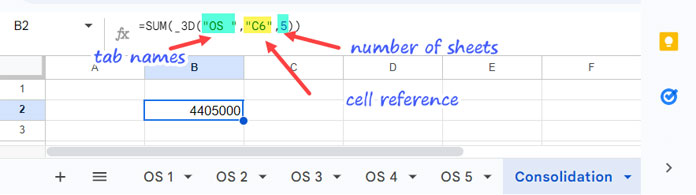

Where "OS " is the common tab name, "C6" is the cell reference, and 5 represents the range of sheets from 1 to 5.

The result will be equal to using the formula ='OS 1'!C6+'OS 2'!C6+'OS 3'!C6+'OS 4'!C6+'OS 5'!C6.

Here is an example of a 3D reference using a REDUCE-based formula in line with the _3D custom function in Google Sheets:

=SUM(
     REDUCE(,ARRAYFORMULA("OS "&SEQUENCE(5)&"!"&"C6"),
     LAMBDA(a,v,IFNA(VSTACK(a,INDIRECT(v)))))
)

What about using a cell range in a 3D reference in Google Sheets?

My custom function or formula can handle cell ranges without any problems. Here are two examples:

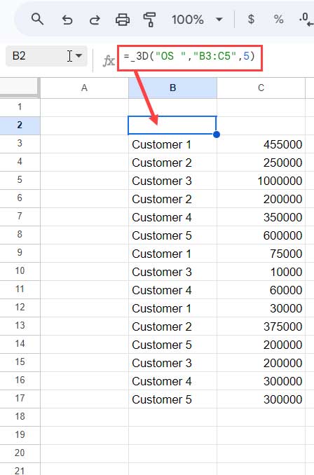
=_3D("OS ","B3:C5",5)

This formula will return the range B3:C5 from all five sheets that start with the tab name "OS ".

Here is the formula alternative to the above _3D custom-named function-based formula.

=REDUCE(,ARRAYFORMULA("OS "&SEQUENCE(5)&"!"&"B3:C5"),
LAMBDA(a,v,IFNA(VSTACK(a,INDIRECT(v)))))

Note: You can use QUERY or other functions to manipulate the results of the 3D range reference.

You have already seen the examples. Here are the syntax, arguments, and how to get the _3D named function.

_3D Named Function: Syntax and Arguments

Syntax:

_3D(sheet_name, cell_range, total_sheets)

Arguments:

sheet_name: The sheet name without the serial number. For example, if the sheets are named “Expense 1”, “Expense 2”, “Expense 3”, and “Expense 4”, then the sheet_name would be "Expense ".

If the sheets are named “Expense1”, “Expense2”, and so on then the sheet_name would be "Expense". I hope you can understand the difference.

cell_range: The cell or range reference to use in the 3-D reference. For example, "C5" or "C5:N100".

total_sheets: The total number of sheets to use. For example, if there are 4 sheets, then the total_sheets would be 4.

FAQs

Q. How do I start using the _3D named function in my Google Sheets?

A. You need to import the function first from the sheet linked below. You can find the instructions here: How to Create Named Functions in Google Sheets.

_3D_Rev0

Q. What are the functions supported in a 3-D reference in Google Sheets?

A. You can use most aggregation functions, lookup functions, QUERY, FILTER, SORT, LET, etc. with 3-D references. The specific functions that work depend on the values in the range you are referencing.

Q. Why does my _3D formula convert dates to numbers?

A. This is because the IFNA function used in the custom function returns the date values as numbers. You can select the cells and format them back to dates by going to the Format menu and clicking Number > Date.

Q. How to remove the blank row at the top of the returned range?

A. Most users will not be affected by this, but if you want to remove it, you can use the QUERY function as follows:

=QUERY(_3D("OS ","B3:C5",5),"SELECT * WHERE Col1 is not null",0)

The Function Behind 3-D Reference in Google Sheets

If you are not a Sheets enthusiast, you can skip this part.

As you can see from the examples under “Examples of 3D Reference in Google Sheets” above, the REDUCE function is the main function behind the _3D named function.

Generic Formula:

REDUCE(,
 ARRAYFORMULA("sheet_name"&SEQUENCE(total_sheets)&"!"&"cell_range"),
 LAMBDA(a,v,IFNA(VSTACK(a,INDIRECT(v))))
)

REDUCE Syntax:

REDUCE(initial_value,
 array_or_range,
 lambda
)

Where:

• initial_value is null.
• array_or_range is the list of sheets generated using an ARRAYFORMULA and SEQUENCE combo.
• lambda:

The INDIRECT function returns the values in the specified range from the first sheet. It is vertically appended using the VSTACK function with the initial value, which is null in the first step.

The REDUCE function passes this result to the initial_value and appends it with the values of the second sheet returned by INDIRECT.

This process continues until REDUCE reaches the last value (Sheet name) in the array_or_range.

That’s all about the 3-D reference in Google Sheets. Thanks for the stay. Enjoy!