To combine data from multiple sheets using IMPORTRANGE, you’ll need to specify the URLs of the sheets in one column and the ranges to import in another column.

We will use the REDUCE LAMBDA function to execute multiple IMPORTRANGE operations at once. This method is user-friendly, and I’ll include a detailed formula explanation.

Features of the formula:

1. You can merge multiple Google Sheets files (workbooks) in one go.
2. The range dimensions don’t need to be equal in size or identical.
3. If a workbook contains multiple sheets, you can import and merge data from selected sheets.

As a side note, we will also use functions like CHOOSECOLS, ARRAYFORMULA, and QUERY. However, the core functions are REDUCE and IMPORTRANGE.

Example: Combining Three Sheets with IMPORTRANGE in a Fourth File

Assume you have three Google Sheets files (workbooks) named sales 1, sales 2, and sales 3, each containing a sheet. The sheet names in each file are “Zone 1,” “Zone 2,” and “Zone 3.”

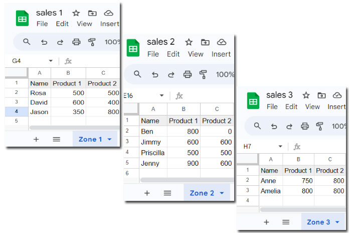
How can you combine these three sheets using the IMPORTRANGE function in a fourth file without writing three separate formulas for each sheet?

Here are the step-by-step instructions. Keep in mind that we are working on the fourth file.

Step 1: Spreadsheet URLs

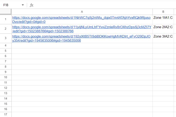
Open sales 1 and copy the URL from the address bar. Navigate to the fourth file and paste the URL into cell A1. Similarly, copy-paste the URLs from the sales 2 and sales 3 files into A2 and A3, respectively.

Step 2: Range Strings

In B1, enter the range to import from the sales 1 sheet. The tab name is “Zone 1,” so if you want to import the range A1:C, enter Zone 1!A1:C in B1.

In B2, enter the range to import from the sales 2 sheet. I am entering Zone 2!A2:C.

The last sheet is sales 3. Enter the range to import from this sheet in B3. I am entering Zone 3!A2:C.

When entering the first sheet range, I included the header row and omitted it in the second and third sheets.

In the next step, we will merge data from these sheets using the entered ranges.

Step 3: Combining Multiple Sheets with IMPORTRANGE

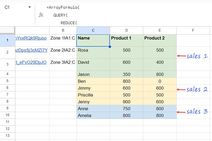
In cell C1, enter the following formula.

=ArrayFormula(
   QUERY(
      REDUCE(
         TOCOL(,1), A1:A3&"|"&B1:B3, 
         LAMBDA(accumulator, url, VSTACK(accumulator, 
            IMPORTRANGE(
               CHOOSECOLS(SPLIT(url, "|"), 1), 
               CHOOSECOLS(SPLIT(url, "|"), 2)
            )
         ))
      ), "SELECT * WHERE Col1 IS NOT NULL"
   )
)

The formula may initially return #REF! errors. Hover your mouse over the cell and click “Allow Access.”

This way, you can combine multiple sheets using IMPORTRANGE in Google Sheets.

Note: If a workbook contains more than one sheet and you want to merge all of them, you need to specify each sheet individually. Copy each URL from the workbook, enter them in column A, and specify the ranges in column B as described above. This is because each sheet in a workbook has its own URL and tab name.

Formula Breakdown

The formula involves several steps. Let me break it down and explain each step. This breakdown is optional, and you can skip it if you prefer.

Before proceeding, replace the open ranges in B1:B3 with closed ranges, such as Zone 1!A1:C5, Zone 2!A2:C5, and Zone 3!A2:C5. Otherwise, you may encounter issues during the process.

1. Combining Spreadsheet URL and Range String

The IMPORTRANGE function takes two arguments: a spreadsheet URL and the range to import as a string.

Syntax:

IMPORTRANGE(spreadsheet_url, range_string)

To merge data from multiple sheets using IMPORTRANGE, we will use the REDUCE function. REDUCE operates on an array, so we need to combine the URLs and range strings into a single array. First, combine the spreadsheet URL in cell A1 with the corresponding range string in cell B1, and then split them for use in IMPORTRANGE.

Formula:

=A1 & "|" & B1

This combines the URL in cell A1 with the range string in cell B1, using “|” as the separator.

2. Using the IMPORTRANGE Formula

We will split the combined URL and range into two parts using the SPLIT function, and use CHOOSECOLS to extract the first and second parts in IMPORTRANGE as follows:

Formula:

=IMPORTRANGE(CHOOSECOLS(SPLIT(A1 & "|" & B1, "|"), 1), CHOOSECOLS(SPLIT(A1 & "|" & B1, "|"), 2))

This imports the data for the URL specified in cell A1 and the range specified in cell B1.

3. Creating an Unnamed Lambda Function Using IMPORTRANGE

Convert the above formula to a lambda function for use with REDUCE to merge multiple workbooks.

Lambda Function:

LAMBDA(accumulator, url, VSTACK(accumulator, IMPORTRANGE(CHOOSECOLS(SPLIT(url, "|"), 1), CHOOSECOLS(SPLIT(url, "|"), 2))))

This function has two parameters: accumulator and url. It vertically stacks the accumulator values with the result of IMPORTRANGE.

The url represents the combined URL and range string, and the accumulator value is initially null. Use this function with REDUCE.

4. The Role of REDUCE in Combining Multiple Sheets with IMPORTRANGE

Syntax:

REDUCE(initial_value, array_or_range, lambda)

• TOCOL(,1) is the initial_value in the accumulator, which represents null.
• A1:A3 & "|" & B1:B3 is the array_or_range argument.
• The lambda function is as defined above.

When using REDUCE, enter it as an array formula to combine URLs and ranges.

Formula:

=ArrayFormula(REDUCE(TOCOL(,1), A1:A3 & "|" & B1:B3, LAMBDA(accumulator, url, VSTACK(accumulator, IMPORTRANGE(CHOOSECOLS(SPLIT(url, "|"), 1), CHOOSECOLS(SPLIT(url, "|"), 2))))))

This formula combines multiple sheets using IMPORTRANGE. Additionally, QUERY can be used to remove empty rows from the result due to open ranges in column B.

Resources

• How to Use IMPORTRANGE Function with Conditions in Google Sheets
• How to Freeze a Cell in Importrange in Google Sheets (Lock a Cell Reference)
• Dynamic Sheet Names in Importrange in Google Sheets
• How to Vlookup Importrange in Google Sheets [Formula Examples]
• How to Use Query with Importrange in Google Sheets
• Importrange Named Ranges in Google Sheets
• Dynamic Column Id in Query Importrange Using Named Ranges
• Relative Cell Reference in Importrange in Google Sheets
• Dynamic Column in Vlookup Importrange Formula in Google Sheets
• Sumif Importrange in Google Sheets – Examples
• IMPORTRANGE to Import Visible Rows in Google Sheets
• How to Control Reloading of Importrange from the Source File in Google Sheets
• IMPORTRANGE Within FILTER Function in Google Sheets
• IMPORTRANGE Result Too Large Error: Solution
• XLOOKUP with Single IMPORTRANGE & LET in Google Sheets