Need to conditionally sum data across two different Google Sheets files? That’s where the combination of SUMIF with IMPORTRANGE in Google Sheets comes in. This tutorial explains how to use these two functions together, why it sometimes fails, and which alternatives work best when the native combo doesn’t.
What Is IMPORTRANGE in Google Sheets?
IMPORTRANGE is a function that allows you to import data from one Google Sheets file to another. It keeps the imported data updated whenever the source changes.
Syntax:
IMPORTRANGE("spreadsheet_url", "range_string")It plays a key role in enabling data consolidation across spreadsheets, but its use within other functions like SUMIF comes with limitations.
Can You Use SUMIF with IMPORTRANGE in Google Sheets?
Yes and no. You can use SUMIF on imported data if that data is in a standalone range (imported into a helper sheet or separate tab). But directly nesting IMPORTRANGE inside SUMIF will return a #N/A error with the message:
“Argument must be a range.”
This is because SUMIF expects its sum_range argument to be a real range like A1:A10 — not a virtual array generated by another function like IMPORTRANGE.
To work around this, you can either:
- Use a helper sheet to import data first and then run
SUMIFon it - Or use alternatives like
SUMPRODUCTorQUERYwithIMPORTRANGE
This guide walks you through all the working solutions.
Example: Using SUMIF on Imported Data (With Helper Tab)
File Setup
- Source File:
OS_Liability> Sheet:Detail - Destination File:
OS_Summary> Sheet:Summary(for import),Sumif_Import(for calculations)
Source Data (Detail!A1:D):
| Customer Name | Bill No. | Outstanding Amount | Aging by Days |
|---|---|---|---|
| A | RA-5 | 25000 | 36 |
| B | RA-6 | 25000 | 40 |
| A | RA-7 | 15000 | 45 |
| A | RA-8 | 15000 | 45 |
| B | RA-9 | 100000 | 90 |
| B | RA-10 | 100000 | 91 |
| A | RA-11 | 100000 | 91 |
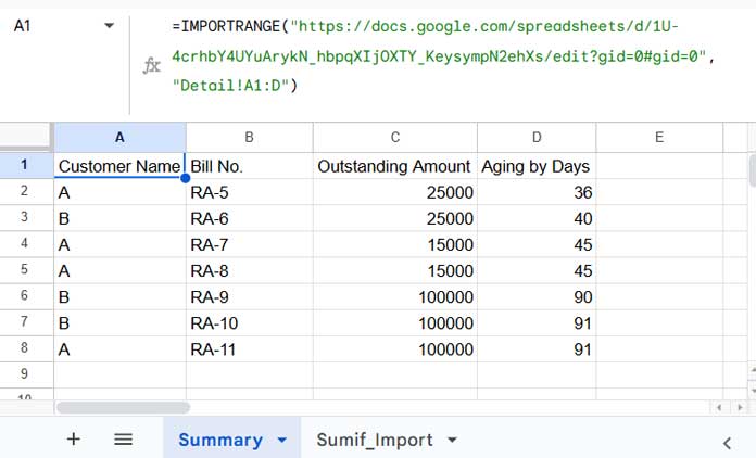
Step 1: Import Data with IMPORTRANGE
In cell Summary!A1 in the destination file:
=IMPORTRANGE("<source-file-URL>", "Detail!A1:D")Click Allow access when prompted.
Step 2: Apply SUMIF to Imported Data
In Sumif_Import, enter:
A1: A
A2: B
B1: =SUMIF(Summary!A:A, A1, Summary!C:C)Then drag the formula down to B2.
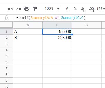
This formula returns the total outstanding amount for the customer name entered in column A. For example, the formula in B1 gives the total outstanding liability for customer “A”.
ArrayFormula: SUMIF Without Dragging Down
Instead of dragging the formula down, you can use the following formula in cell B1 to spill down to B2:
=ArrayFormula(SUMIF(Summary!A:A, A1:A2, Summary!C:C))This reduces the number of formulas required when handling multiple criteria.
SUMIF with IMPORTRANGE – Alternatives That Work Without Helper Tabs
Many users prefer not to use helper sheets. Here are two practical alternatives that avoid that.
Option 1: SUMPRODUCT with IMPORTRANGE
Instead of using SUMIF, use this SUMPRODUCT-based combination:
=LET(
  import, IMPORTRANGE("<source-file-URL>", "Detail!A1:D"),
  SUMPRODUCT(CHOOSECOLS(import, 1) = A1, CHOOSECOLS(import, 3))
)
This formula returns the sum of values in column 3 (Outstanding Amount) where column 1 (Customer Name) matches the value in A1. Drag it down to apply the same logic to other customer names listed in A2, A3, and so on.
How it works:
IMPORTRANGE(...)brings the data from the source sheet.LETstores that imported array in a variable namedimport.CHOOSECOLS(import, 1)extracts the first column (criteria range).CHOOSECOLS(import, 3)extracts the third column (sum range).SUMPRODUCT(...)then multiplies the Boolean match array with the corresponding values, summing only those that match the condition.
Multiple Criteria Version
Instead of dragging down the above formula for each condition, you can use the following version to spill results based on the list in A1:A2:
=LET(
  import, IMPORTRANGE("<source-file-URL>", "Detail!A1:D"),
  MAP(A1:A2, LAMBDA(r, SUMPRODUCT(CHOOSECOLS(import, 1) = r, CHOOSECOLS(import, 3))))
)
This method is fast and flexible — and works well without any helper sheets.
Option 2: QUERY with IMPORTRANGE
Instead of using SUMIF, use this QUERY-based combination:
=QUERY(
  IMPORTRANGE("<source-file-URL>", "Detail!A1:D"),
  "SELECT SUM(Col3) WHERE Col1='"&A1&"' LABEL SUM(Col3)''"
)
This returns the sum of column 3 where column 1 matches A1. Drag this formula down to apply it to additional criteria.
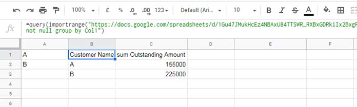
Lookup-Specific Results
Instead of dragging down the query, you could use this formula to look up the condition in column A and display results next to a custom list of customer names:
=ArrayFormula(
  VLOOKUP(
    A1:A2,
    QUERY(IMPORTRANGE("<source-file-URL>", "Detail!A1:D"),
    "SELECT Col1, SUM(Col3) WHERE Col1 IS NOT NULL GROUP BY Col1"),
    2,
    0
  )
)
Multi-Group Summary Using QUERY
To summarize all customer names without typing each one manually:
=QUERY(
  IMPORTRANGE("<source-file-URL>", "Detail!A1:D"),
  "SELECT Col1, SUM(Col3) WHERE Col1 IS NOT NULL GROUP BY Col1"
)
This replaces SUMIF and gives a grouped total per name.
Final Thoughts: Which Method to Use?
- Use SUMIF with a helper tab if you want simplicity and don’t mind importing data visibly.
- Use SUMPRODUCT + IMPORTRANGE if you want everything in one cell.
- Use QUERY + IMPORTRANGE for more powerful grouping or summaries.
Each method lets you conditionally sum values from another file, and all avoid the frustrating “Argument must be a range” error.


I got lost here when you used Col3 and Col1 in this formula.
=query(importrange("insert URL","Detail!A1:D"),"Select sum(Col3) where Col1='"&A1&"' label sum(Col3)''")
I used your formula but still got a parse error
=query(importrange("URL","Sales!C7:M"),"Select sum("Sales"!I7:I) where Col5='"&E4&"' label sum("Sales"!I7:I)''")
I want to calculate the sum from a particular column taken from another Google Sheet file based on a criterion and month.
Hi, Paul Santos Estrella,
Assume you have imported 5 columns from P1:T. To sum the range
R1:R, usesum(Col3)notsum(R1:R).Col3 represents column # 3.
It works. But when I drag the formula, it gives me the same value.
Could you help me with this, please?
Hi, Vienna,
Let me try. Share the URL of a sample via reply below.