You can use the ampersand to join columns and criteria to code a multiple criteria Sumif formula. The criteria can be from one column or two or more different columns. Sumif supports multiple column criteria in Google Sheets.

I have used this trick in an earlier post. The link I have included in the later part of this guide. But that post was not specifically handling this topic. So I thought I should write this tutorial separately as it can be useful for newbies.

To code a multiple criteria Sumif formula in Google Sheets, you should use the function ArrayFormula together with Sumif. Another requirement is the use of the& that joins multiple criteria and corresponding columns.

Why don’t you use the Sumifs instead?

The reason Sumifs formula can’t expand. In other words, it returns a single cell output.

Here you are going to find the benefits of using Sumif with multiple conditions in Google Sheets.

But there’s is a shortfall in using multiple criteria in Sumif using the Ampersand. It won’t work with comparison operators in Sumif. I mean a date difference as the condition in Sumif formula is not possible this way.

How to Use Multiple Criteria in Sumif in Google Sheets

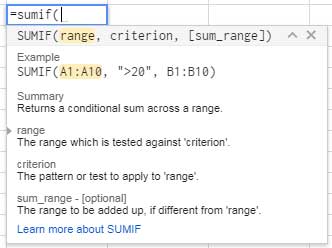
Let me begin with the Sumif Syntax in Google Sheets:

I know you are not new to Sumif. Still here is a basic example meant for those who are inexperienced in the use of the Sumif function in Google Sheets.

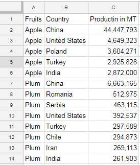
Sample Data:

Formula:

=sumif(A1:A,"Plum",C1:C)

This single criterion Sumif formula sums column C if the value in column A is “Plum”.

There is no issue in using multiple criteria in Google Sheets Sumif in a single column. As an example, see how I am using the Sumif formula to sum the value of both “Plum” and “Apple”.

=ArrayFormula(sum(sumif(A1:A,{"Plum","Apple"},C1:C)))

This multiple condition Sumif formula has already found a place on my earlier detailed tutorial – How to Sumif When Multiple Criteria in the Same Column in Google Sheets.

When the criteria in Sumif are in two different columns, either you should use the Sumifs function or Sumif combination formula.

Here is that ArrayFormula + Sumif + Ampersand combination.

Multiple Criteria Sumif Formula in Google Sheets

See how I am coding a multiple criteria Sumif formula in Google Sheets.

The two criteria that I have used in this example formula are from the column A (“Apple”) and B (“United States”). So the column A1: A and B1: B is combined in the Sumif ‘range’.

In other words, to use multiple criteria from two or more different columns in Sumif you should follow the below two tips.

1. Combine the criterion using the ampersand (E2&F2).

2. Combine the corresponding columns to the criteria similarly (A1:A&B1:B).

Multiple Criteria Sumif Formula – Morethan One Criteria in Same Column + Additional Column

You can read OR condition (criteria in the same column) + AND condition (criterion in a different column)

This is also possible using Sumif in Google Sheets! Further, it has an edge over Sumifs. So it’s necessary for me to first show you the Sumifs formula.

Sum column C;

1. If column A contains either of the item “Apple” or “Plum”.

2. The column B contains “United States”.

Formula:

=ArrayFormula(sumifs(C2:C,B2:B,"United States",regexmatch(A2:A,"Apple|Plum"),TRUE))

This formula depends on the mighty Regexmatch in Google Sheets. If you do not use Regex, you may then nest the Sumifs which is not an ideal solution.

Want a formula explanation?

Must Read: Regexmatch in Sumifs in Google Sheets.

Now see the multiple criteria Sumif formula (OR, AND in Sumif) that is equivalent to the above Sumifs.

=ArrayFormula(SUM(sumif(A1:A&B1:B,{"AppleUnited States","PlumUnited States"},C1:C)))

The above multiple criteria Sumif formula would be slightly different in use if the conditions are in cells not within the formula.

In such cases, you should know how to format the conditions. See how I have presented the conditions in the range E2: F3 and used in the formula.

There is a clear benefit of using Sumif over Sumifs in multiple conditions in the same or different columns.

The Benefit of Using Multiple Criteria Sumif Formula in Google Sheets

To understand the benefit of Sumif as above in multiple conditions, just remove the Sum in the formula.

You can see that it produces an array result. Unlike Sumifs, Sumif can produce an array result.

Similar: Sumifs Array Formula Expanding Issue and Alternative Formulas.

With this example, I am concluding this tutorial on the multiple criteria Sumif formula usage in Google Sheets. Thanks for the stay.