There are a total of six comparison operators in Google Sheets, along with corresponding comparison functions.

The comparison operators are “=”, “<“, “<=”, “>”, “>=”, and “<>”. In Google Sheets, certain functions serve as equivalents to these comparison operators.

These functions are EQ, LT, LTE, GT, GTE, and NE. In this guide, I will explain how to use both the comparison operators and their equivalent functions in Google Sheets.

I primarily use comparison operators in formulas, as I became accustomed to them when transitioning from Excel to Google Sheets. The comparison functions are secondary in importance to me.

Usage of Comparison Operators in Google Sheets and Alternative Functions

You can employ comparison operators in Google Sheets with various types of values, such as text, numeric, dates, tick boxes, characters, special characters, etc.

It’s important to note that the outputs of these comparison operators are Boolean values, either TRUE or FALSE.

Google Sheets Comparison Operator “=” and Function EQ (Equal)

“=” Operator: Use this operator or the EQ function for an equality test.

Here is an example to help you understand how to use the comparison operator “=” and its alternative function EQ.

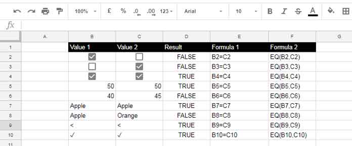
You can obtain the formula output in Column D by using the formulas in Column E or F.

Note: The tick box has the value of TRUE when ticked and FALSE if not.

For instructions on how to insert Tick Boxes in Google Sheets, please follow the link below.

Must Read: Insert Checkboxes and Tick Marks in Google Sheets

The EQ (Equal To) Function Syntax:

EQ(VALUE1, VALUE2)

Common Usage of “=” Operator in Spreadsheets:

All the comparison operators are most commonly used with the IF logical statement.

If you want to learn how to use the “=” operator or the EQ function with IF, here’s an example:

=IF(B2=C2, "YES", "NO")

The above is a commonly used formula. You can replace the same formula with the one below, where the “=” operator is replaced by the EQ function.

=IF(EQ(B2, C2), "YES", "NO")

Google Sheets Comparison Operator “<” and Equivalent Function LT (Less Than)

“<” Operator: Use this operator or the LT function to test if the first value is less than the second value.

Example of the use of the “<” operator and LT function:

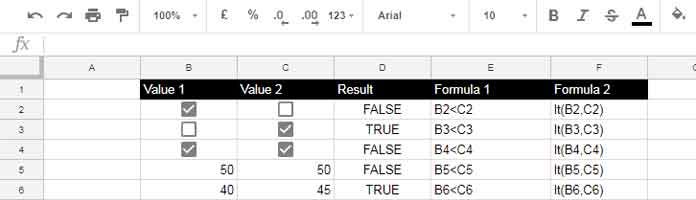
Similar to my first example, you can use either the “<” operator or the LT function to check whether the values in Column B are less than the values in Column C.

The first three rows in the range contain tick boxes. I’ve already explained above how to add tick boxes to cells.

Please note that the value of Boolean TRUE is 1, and FALSE is 0. This should be considered alongside the fact that the tick box returns TRUE when it’s ticked and FALSE otherwise.

LT (Less Than) Function Syntax:

LT(VALUE1, VALUE2)

Common Usage of “<“:

Undoubtedly, all the comparison operators are commonly used with IF or IFS. Here is one such use.

=IF(B2<C2, "YES", "NO")

The above formula uses the “<” comparison operator, and the below formula is the equivalent using the LT function.

=IF(LT(B2, C2), "YES", "NO")

Note: I am not suggesting that these operators are only for use with IF or IFS. You can employ comparison operators in Google Sheets in QUERY, FILTER, and various other functions.

Google Sheets Comparison Operator “<=” and Function LTE (Less Than or Equal To)

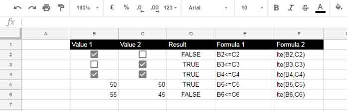
“<=” Operator: Use this operator or the LTE function to test if the first value is less than or equal to the second value.

You can utilize the “<=” operator similarly to the “<” operator, and it applies to the LTE function as well.

The LTE (Less Than or Equal To) Function Syntax:

LTE(VALUE1, VALUE2)

Common Usage of ‘<=’:

Consider this logical test.

=IF(B2<=C2, "YES", "NO")

The same formula without using the comparison operator:

=IF(LTE(B2, C2), "YES", "NO")

Google Sheets Comparison Operator “>” and Function GT (Greater Than)

“>” Operator: Use this operator or the GT function to test if the first value is greater than the second value.

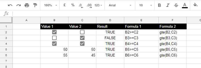
In the example below, the formulas test whether the values in Column B are greater than the values in Column C.

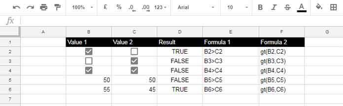
The “>” comparison operator tests the value in Column B against the value in Column C. If the values in Column B are greater than the values in Column C, the formulas return TRUE; otherwise, they return FALSE.

You can find the formulas in column E and Column F. In column D, use any of the formulas as both are similar.

GT (Greater Than) Function Syntax:

GT(VALUE1, VALUE2)

Common Usage of “>”:

Let’s see how to use the GT function as well as the “>” with the IF function.

The formula using “>”:

=IF(B2>C2, "YES", "NO")

The Formula using the GT function:

=IF(GT(B2, C2), "YES", "NO")

Google Sheets Comparison Operator “>=” and Function GTE (Greater Than or Equal To)

“>=” Operator: Use this operator or the GTE function to test if the first value is greater than or equal to the second value.

See this example.

I am testing the values in Column B with Column C. What I want is if the values in Column B are greater than or equal to the values in Column C, I want the formulas to return TRUE; otherwise, they should return FALSE.

In column E, I’ve used the “>=” operator-based formulas, and in Column F, the GTE function-based ones. You can use either of these formulas in column D.

The GTE (Greater Than or Equal To) Function Syntax:

GTE(VALUE1, VALUE2)

Common Usage of “>=”:

The usage of the GTE function as well as the “>=” with the IF function.

The formula using “>=”:

=IF(B2>=C2, "YES", "NO")

The Formula using the GTE function:

=IF(GTE(B2, C2), "YES", "NO")

Google Sheets Comparison Operator “<>” and Function NE (Not Equal To)

“<>” Operator: Use this operator or the NE function for a non-equality test.

When you want to check whether the value in one cell is not equal to the value in another cell, you can use the “<>” comparison operator in Google Sheets or the similar function NE.

See the examples below to understand how to use the “<>” or NE function in Google Sheets.

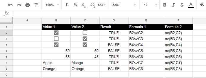
To understand the formulas, take the values in B8 and C8 as an example. The formula in D8 returns FALSE since the values in B8 and C8 are equal.

You have the freedom to choose either of the formulas – the formula using the “<>” operator or the NE function.

The NE (Not Equal To) Function Syntax:

NE(VALUE1, VALUE2)

Common Usage of “<>”:

I am going to use the “<>” comparison operator and NE function with IF.

The formula using “<>”:

=IF(B2<>C2, "YES", "NO")

The Formula using the NE function:

=IF(NE(B2, C2), "YES", "NO")

Utilizing Comparison Operators in Array Formulas

When employing the above operators or functions in an array, you may want to use the ARRAYFORMULA function with them:

=ArrayFormula(IF(D2:D10>E2:E10, "✓", "x"))
=ArrayFormula(IF(GT(D2:D10, E2:E10), "✓", "x"))

The above formulas test whether the values in D2:D10 are greater than E2:E10 and return a tick mark if the formula evaluates to TRUE; otherwise, it returns an ‘x’ mark.

This approach applies to all the comparison operators and equivalent functions.

Conclusion

I’ve observed that Google Sheets users frequently employ comparison operators in formulas rather than the equivalent functions. The choice between them is yours.

Furthermore, Google Sheets includes a function called ISBETWEEN, which you can utilize to determine if a value falls between two other values. For more information, refer to the resources provided below.

1. Simple Comparison Operators in Google Sheets Query
2. How to Use Isbetween with Filter Formula in Google Sheets
3. Countifs with Isbetween in Google Sheets