To create a SUMIFS array formula that expands results, you’ll need to use a Lambda function in Google Sheets.
SUMIF can expand results using the ARRAYFORMULA function, but SUMIFS cannot. One limitation of SUMIF is that it can only handle a single criteria range.
However, in SUMIF, we can combine criteria and criteria ranges as an alternative solution to the SUMIFS array formula issue. This approach doesn’t always work, especially when dealing with date ranges as criteria.
Another workaround is to utilize QUERY. This method may also have some limitations akin to those of SUMIF. I will cover all of these methods and tips in this tutorial.
SUMIFS Array Formula for Expanded Results in Google Sheets
This example demonstrates the use of date range criteria in a SUMIFS array formula in Google Sheets.
Here is the syntax of SUMIFS for your reference:
SUMIFS(sum_range, criteria_range1, criterion1, [criteria_range2, …], [criterion2, …])Let’s assume you have the delivery dates of various products in column A, their quantities in column B, and the delivery confirmations in column C. An “x” mark in column C signifies that the delivery of that product has been confirmed by the vendor.
In this scenario, you want to calculate the total confirmed deliveries between 01/11/2023 and 05/11/2023. The criteria for these two dates are in cells D2 and E2, and another criterion, “x,” is in cell F2.
Additionally, there is another set of criteria in cells D3:F3, which is 06/11/2023 and 10/11/2023 in cells D3:E3 and “x” in cell F3.
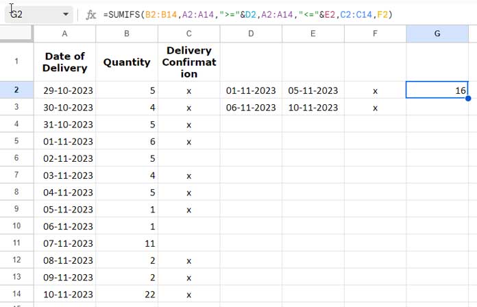
Here is the non-array SUMIFS formula in cell G2:
=SUMIFS(B2:B14,A2:A14,">="&D2,A2:A14,"<="&E2,C2:C14,F2)To expand the results in cells, we need to use a SUMIFS array formula.
In Microsoft 365 Excel, the formula expands due to its dynamic array behavior. You simply specify the criteria range in the formula as follows:
=SUMIFS(B2:B14,A2:A14,">="&D2:D3,A2:A14,"<="&E2:E3,C2:C14,F2:F3)This won’t work using SUMIFS in Google Sheets. Here is how to use a SUMIFS array formula to expand its result in Google Sheets.
SUMIFS with MAP Lambda for Expanding Array Results
First, let me explain how to easily convert a non-array SUMIFS formula into a SUMIFS array formula using the MAP lambda function in Google Sheets:
You should specify the criteria ranges within MAP individually, name them within the Lambda function, and replace the existing criteria in SUMIFS with assigned names.
The criteria range in this case are D2:D3, E2:E3, and F2:F3.
Specify them with MAP as follows:
=MAP(D2:D3,E2:E3,F2:F3, LAMBDA(criterion1, criterion2, criterion3, sumifs_formula)Replace sumifs_formula with the non-array formula and in that replace D2 with criterion1, E2 with criterion2, and F2 with criterion3.
Here is the resulting SUMIFS array formula for expanding results:
=MAP(D2:D3,E2:E3,F2:F3, LAMBDA(criterion1, criterion2, criterion3, SUMIFS(B2:B14,A2:A14,">="&criterion1,A2:A14,"<="&criterion2,C2:C14,criterion3)))Anatomy of the Formula
Let’s dissect the components of the formula to help you understand the logic:
Syntax of the MAP Function:
MAP(array1, [array2, …], LAMBDA([name, …], formula_expression))In our formula, the arguments are as follows:
array1: D2:D3array2: E2:E3array3: F2:F3
Within the LAMBDA function:
name(s): criterion1, criterion2, criterion3 (corresponding to array1, array2, and array3)formula_expression:SUMIFS(B2:B14, A2:A14, ">="&criterion1, A2:A14, "<="&criterion2, C2:C14, criterion3)
The MAP function applies the LAMBDA function for each set of criterion1, criterion2, and criterion3 provided in D2:D3, E2:E3, and F2:F3, respectively.
This results in a list of sums based on these different sets of criteria.
SUMIFS Array Formula Alternatives
The above SUMIFS array formula is not easy to replace with regular formulas. Therefore, I recommend sticking with it.
However, in certain scenarios, you can consider using other formulas as alternatives to the SUMIFS array formula. Here are a few examples.
SUMIF (Criteria in Single Column)
If you want to apply multiple criteria within a single column, you can use SUMIF, which has the capability to expand results.
Here is the syntax of SUMIF for your reference:
SUMIF(range, criterion, [sum_range])Problem:
Summing sales in Q1 (E3) and Q2 (E4) when the quarters are specified in A2:A and the sales amounts are specified in C2:C.
Solution:
=ARRAYFORMULA(SUMIF(A2:A9,E3:E4,C2:C9))
SUMIF (Criteria in Multiple Columns)
This time, we have month names (in text) in column A, fruit names in column B, and sales amounts in column C.
The objective is to calculate the sum of sales for the fruits Apple and Orange in January separately.
The criteria are set as follows:
- E3 and E4 contain “January”
- F3 and F4 contain “Apple” and “Orange”
Formula:
=ARRAYFORMULA(SUMIF(A2:A&B2:B,E3:E4&F3:F4,C2:C))
Since SUMIF can handle criteria in a single column, we have combined criteria in two columns along with their respective ranges.
However, it’s essential to note that this SUMIF-based array formula alternative may not work in all scenarios, particularly when dealing with criteria involving comparisons.
Here is the MAP + SUMIFS alternative:
=MAP(E3:E4,F3:F4,lambda(criteriaSet1,criteriaSet2, sumifs(C2:C,A2:A,criteriaSet1,B2:B,criteriaSet2)))Using QUERY as an Alternative to SUMIFS for Expanding Array Results
QUERY is one of the best functions for data manipulation and visualization.
The output of the QUERY can be structured, making it useful for creating formula-based Pivot Tables and charts.
Here is an example of how to address the SUMIFS array formula expansion issue with a QUERY formula. We will use the fruit’s data as an example here.
Formula:
=QUERY(A2:C,"Select A,B, sum(C) where A Matches 'January' and B matches 'Apple|Orange' group by A,B label sum(C)''")Please note that this formula is case-sensitive, and I’ve specified the criteria as hard-coded values.
Conclusion

In certain scenarios, you might want to use the ARRAYFORMULA function with SUMIFS, not to expand the results but to expand a function used within it, especially for date-related functions.
Here is an example:
=ARRAYFORMULA(SUMIFS(C2:C,YEAR(A2:A),F2,B2:B,E2)In the above example, you can see the YEAR date function. Since it is a non-array function, you should use ARRAYFORMULA with the SUMIFS.
Actually, the ARRAYFORMULA is used to support the YEAR function. That means you can also use the above formula as follows.
=SUMIFS(C2:C,ARRAYFORMULA(YEAR(A2:A)),F2,B2:B,E2)


Hey Guys,
I have a problem combining two formulas. Maybe you can help me with my problem.
1.
=SUMIF($S$5:$NT$5;”<"&today();S20:NT20)2.
=ARRAYFORMULA(sum(iferror(value(regexextract(substitute(;".";"");"[0-9,]+")))))+(COUNTIFS(S20:NT20;{"u"})*7,5)+(COUNTIFS(S20:NT20;{"k"})*7,5)+(COUNTIFS(S20:NT20;{"su"})*7,5)+(COUNTIFS(S20:NT20;{"kk"})*7,5)+(COUNTIFS(S20:NT20;{"ü"})*7,5))Example Situation is:
I have two shift systems where I have to show the work hours spent.
In the first shift system, I have only numbers that have to be summed.
In the second, I have letters and numbers in the cells (MO7,5, EV7,5, and so on).
I have a problem combining these two formulas to get the work hours spent until today in the second shift system.
Hopefully, you can help me
Sebastian
Hi, Sebastian,
I don’t understand the issue of combining them. It may be due to the regex text function in the second formula. So you may wrap that formula with VALUE()
If that doesn’t work for you, please feel free to share a sample sheet in the ‘reply’ below.
Prashanth, Many thanks. Very grateful for people like you.
I have a header row of dates (starting at N1), e.g.,
Apr 18, 2022 | Apr 25, 2022 | May 02, 2022 | May 09, 2022|…|Dec 26, 2023
From N2:2-N1000:1000 I have numeric values.
I need to sum the numbers when N1:1>TODAY().
The current sumifs formula (in each row as I can’t use ARRAYFORMULA) is as follows:
=if(len(A2)>0, sumifs(N2:2,N$1:EZ$1,">="&TODAY())*5*8,"")Would you be able to steer me in the right direction to change and allow this functionality to work within an ARRAY?
Hi, MC,
I’ve posted a similar solution here – Get the Last 7, 30, and 60 Days Total in Each Row (from Today) in Google Sheets.
Here is a customized formula for you.
=ArrayFormula(if(A2:A="",,dsum(transpose({A2:A,filter(N2:1000,N1:1>=today())}),
sequence(rows(A2:A)),{if(,,);if(,,)})*40))
To know the last part, i.e.,
{if(,,);if(,,)}, please check this guide – Two Ways to Specify Blank Cells in Google Sheets Formulas.Hi,
I am trying to do a SUMIF for unique values. I want to get the sum of column 4 based on the unique values of columns B, C, and D.
E.g.
Column A | Column B | Column C | Column D | Column E | Column F
Jan | Week 1 | Mays | Order 1 | Chair | $20
Hi, Chang,
Your description of the problem and sample data doesn’t match.
I think you want to sum column F after making unique columns B, C, and D. If so, you can try this Query.
=query(A1:F,"Select B,C,D,sum(F) where A is not null group by B,C,D label sum(F)''")Do give four columns and enough rows for this formula to return a summary report.
Using Sumif as Sumifs is amazing..! Solved my problem 🙂 Thank you.
Hi, this scenario is driving me nuts if I want to convert to kind of arrayformula
For example:
A;B;C
1;100;1
2;300;2
3;300;1
4;500;1
5;200;2
when if using =SUMIFS(B$2:B,C$2:C,C2,A$2:A ,”<"&A2), on every row from 2nd row in Column D, results in:
A;B;C;D
1;100;1;0
2;300;2;0
3;300;1;100
4;500;1;400
5;200;2;300
Please give some magic one liner formula for this scenario:
Thank you so much!
Hi, Kris,
I don’t have a ‘magic one-liner formula’ at least for now 🙁
But if you have only 2 or 3 unique values in column C, then you can follow the below workaround formulas.
Step 1:
Insert this filter in cell F2 which will populate the data in F2:H.
=filter($A$2:$C$6,$C$2:$C$6=1)Step 2:
Key in the below Sumif Array in cell I2.
=ArrayFormula(If(len(H2:H),(SUMIF(F2:F,"<"&F2:F,G2:G)),))Step 3:
The formula to insert in cell K2 to populate data in K2:M.
=filter($A$2:$C$6,$C$2:$C$6=2)The formula to be inserted in cell N2;
=ArrayFormula(If(len(M2:M),(SUMIF(K2:K,"<"&K2:K,L2:L)),))This is when there are 2 unique values in column C (1 and 2). If more than two unique values, you may want to repeat the filter and Sumif accordingly.
Note: Make sure that column A is sorted in ascending order. Later if you want you can Vlookup these outputs to your column D. I am skipping that part.
Best,
For me, the below works when I use it on the same sheet.
=ArrayFormula(sumif(E2:E569,unique(E2:E569),C2:C569))But I want it to work in a different sheet with a reference sheet name as ‘RAW DATA’.
I have tried using the below formula, but not working:
=ArrayFormula(SUMIF('Raw Data'!E2:E569,UNIQUE(E2:E569),C2:C569))Kindly help!
Hi, Pratick Das,
You were so close to a working SUMIF array solution!
=ArrayFormula(SUMIF('Raw Data'!E2:E569,UNIQUE('Raw Data'!E2:E569),'Raw Data'!C2:C569))Best,
You are a genius!
Can you post the example sheet used for these examples? Would really appreciate the SUMIF in ARRAYFORMULA one, as I’m trying to recreate it currently.
Hi, Blake,
See the below link.
https://docs.google.com/spreadsheets/d/1Hit4kL8Ex9vvqakShfaDlILwzLFDPRL2im7N3MrDs5g/copy
Hi,
I’m struggling with getting ARRAYFORMULA with SUMIFs. I’ve tried using QUERY but it gives me “sum” text instead of sum. I hope that you could help me.
I have an array:
column A – date from
column B – date to
column C – number
I have a second array:
column E – date
column F – empty
I want to put the sum of all numbers from column C if date from column E is between dates from columns A and B.
It works for one row:
=SUMIFS(C:C, A:A, "=" & E3)Of course, it will not ARRAYFORMULA:
=ARRAYFORMULA(SUMIFS(C:C, A:A, "=" & E1:E))It produces the result for only one row.
This query gives me “sum” instead of a real sum:
=QUERY(A1:C1, "select SUM(C) where A = '"&E1&"'")So how to rewrite these formulas so it would work for all the rows to avoid copying the SUMIFS formula to each row?
Thanks a lot in advance for any help.
Hi, Cezary,
You want a SUMIF/SUMIFS array formula in a date range. That is possible with an MMULT function based formula.
I have already detailed that in this post – Array Formula to Conditionally Sum Date Ranges in Google Sheets.
But for your custom need, I have tweaked the formula detailed in that tutorial as below.
=ArrayFormula(if(len(E2:E),mmult((E2:E>=transpose(A2:A))*((E2:E<=transpose(B2:B))),n(C2:C)),))Possibly you can use this formula in cell F2 (as per your explanation of the problem above).
Further, I have my example Sheet ready for you HERE.
Best
Magic 🙂 Thanks a ton!