Calculate Last 7, 30, and 60 Days Total in Each Row of Google Sheets

When you have daily data arranged in columns (dates across the top), you may want to calculate a rolling total. For example, the last 7, 30, or 60 days total in each row.

In this tutorial, I’ll show you how to do this in Google Sheets using SUMIFS. I’ll also cover how to make it auto-expand with LAMBDA, and finally, share one older formula approach for reference.

Table of Contents

Sample Data

Here’s a simple layout to explain the problem:

Item	15/08/25	16/08/25	17/08/25	18/08/25	19/08/25	…	24/08/25
A	1	2			1	…	1
B	1			3		…
C	1		1	1	2	…	1

Dates are in row 2 (D2:M2).
Values start from row 3 (D3:M).
Totals will go in column A.

I’ve prepared a sample sheet that you can copy and experiment with:

Copy Sample Sheet

Formula for Last 7 Days

The first thing you need to decide is: do you want to include today in the calculation, or only count completed days? The formula is almost the same, but the condition changes slightly.

Formula Including Today

In A3 enter:

=SUMIFS(D3:3, $D$2:$2, ">"&TODAY()-7, $D$2:$2, "<="&TODAY())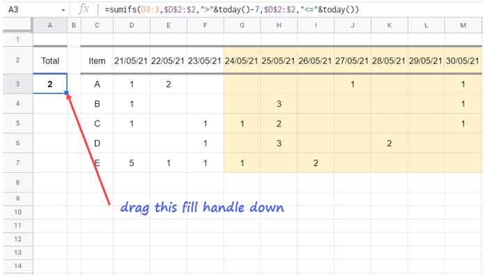

Google Sheets SUMIFS formula dragged down to calculate last 7 days total in each row

This totals the last 7 days including today for row 3. Drag down to fill other rows.

Formula Excluding Today

If you don’t want today’s data included (say it’s incomplete):

=SUMIFS(D3:3, $D$2:$2, ">="&TODAY()-7, $D$2:$2, "<"&TODAY())

This gives the last 7 days excluding today.

Tip: In real use, your range will often be open-ended across columns (D3:3). But if you prefer, you can limit it (e.g., D3:M3 for values and $D$2:$M$2 for headers).

Auto-Expanding with LAMBDA

Dragging down works fine, but if you want a formula that spills results automatically for all rows, use BYROW with LAMBDA.

LAMBDA Formula Including Today

=BYROW(D3:1000, 
   LAMBDA(row, LET(total, 
      SUMIFS(row, D2:2, ">"&TODAY()-7, D2:2, "<="&TODAY()), 
      IF(total=0,,total))
   )
)

Quick note: BYROW feeds each row into the LAMBDA. Inside, SUMIFS checks the dates in row 2 and totals the values that fall within the last 7 days. With LET, I’m just saving that total into a name so I can reuse it. Finally, the IF(total=0,,total) keeps things neat by skipping empty rows.

LAMBDA Formula Excluding Today

=BYROW(D3:1000, 
   LAMBDA(row, LET(total, 
      SUMIFS(row, D2:2, ">="&TODAY()-7, D2:2, "<"&TODAY()), 
      IF(total=0,,total))
  )
)

This way you don’t need to copy formulas down manually. The little trick with IF(total=0,,total) hides trailing zeros when your rows are blank.

Important: Put the formula in A3 after clearing column A. Don’t insert it elsewhere, or you may end up with extra blank rows at the bottom.

Last 30 and 60 Days

Once you get the last 7 days working, the 30 and 60 day totals are just as simple. Replace -7 with -30 or -60.

30 Days Formula Including Today

=SUMIFS(D3:M3, D2:M2, ">"&TODAY()-30, D2:M2, "<="&TODAY())

30 Days Formula Excluding Today

=SUMIFS(D3:M3, D2:M2, ">="&TODAY()-30, D2:M2, "<"&TODAY())

60 Days Formula Including Today

=SUMIFS(D3:M3, D2:M2, ">"&TODAY()-60, D2:M2, "<="&TODAY())

60 Days Formula Excluding Today

=SUMIFS(D3:M3, D2:M2, ">="&TODAY()-60, D2:M2, "<"&TODAY())

For the LAMBDA version, just swap out -7 for -30 or -60.

Bonus: Before LAMBDA

Before LAMBDA and BYROW were available, people used different workarounds to calculate rolling totals across rows. One option was to use DSUM.

Here’s an example formula to calculate the last 7 days total:

=ArrayFormula(
  DSUM(
     {TRANSPOSE(D3:D1000); TRANSPOSE(FILTER(D3:1000, D2:2>TODAY()-7, D2:2<=TODAY()))}, 
     SEQUENCE(ROWS(D3:D1000)), 
     {IF(,,); IF(,,)}
  )
)

How the Formula Works

Database part
{TRANSPOSE(D3:D1000); TRANSPOSE(FILTER(D3:1000, D2:2>TODAY()-7, D2:2<=TODAY()))}
→ This is building a temporary database for DSUM.
→ The FILTER picks only the columns where the date headers fall within the last 7 days.
→ TRANSPOSE flips those values so rows become columns (since DSUM can only total columns, not rows).
→ The extra row we stick on top (TRANSPOSE(D3:D1000); …) acts as a fake header row — DSUM won’t run without one.

Field part
SEQUENCE(ROWS(D3:D1000))
→ Generates a list of “field numbers” automatically.
→ Each number points DSUM to one of the transposed rows, so it totals row-by-row.

Criteria part
{IF(,,); IF(,,)}
→ These are just dummy criteria. DSUM needs a criteria block to work, even if it’s blank.

So the whole trick is: flip the rows into columns, give DSUM a fake header row, feed it field numbers, and let it sum back down again.

The output is the same rolling total per row — but compared to today’s clean SUMIFS + LAMBDA, this method is heavier and harder to debug.

Variations

For the last 30 days, replace -7 with -30.
For the last 60 days, replace -7 with -60.
To exclude today, swap <=TODAY() with <TODAY() and >TODAY()-7 with >=TODAY()-7 (same idea for -30, -60, etc.).

Wrapping Up

Use SUMIFS if you’re fine dragging the formula down.
Use BYROW + LAMBDA if you want one formula that auto-expands.
Decide whether to include today or not, depending on whether today’s data is complete.
Replace -7 with -30 or -60 to change the rolling window.

With these methods, you can build dynamic rolling totals per row that always stay up-to-date.