Want to filter data by drop-down selection such as this week, last week, 2 weeks ago, 3 weeks ago, and so on in Google Sheets? You’re in the right spot.
I’ve covered everything from creating a dynamic week selector drop-down for this purpose to providing step-by-step instructions to implement my formula. In addition, you will find a breakdown of the formula.
For this example, we will use three sheets:
- A database sheet named ‘db’.
- A sheet to apply the drop-down menu and the filter formula called ‘dashboard’.
- A third sheet called ‘helper’ for drop-down values.
All within the same file.
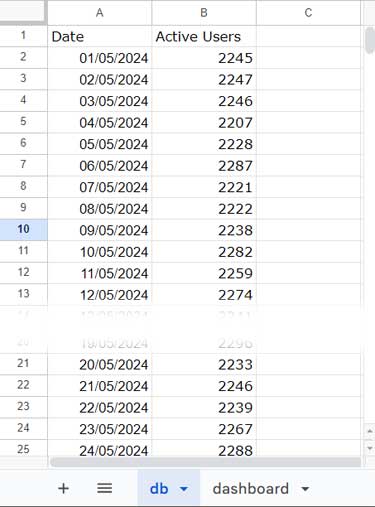
The sample data in the ‘db’ sheet consists of dates in column A and the number of active users of a blog in column B, where A1 and B1 are field labels for ‘Date’ and ‘Active Users,’ respectively.
Set Up a Dynamic Week Selector
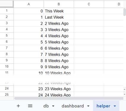
In cell A1 of the ‘helper’ sheet, enter the following formula:
=SEQUENCE(52, 1, 0)This formula creates a sequence of numbers from 0 to 52, representing weeks. You can adjust the number 52 to control how many weeks appear in the drop-down.
In cell B1, enter the following formula to add specific texts to week numbers.
=ArrayFormula(IF(A:A="", ,IF(A:A=0, "This Week", IF(A:A=1, "Last Week", A:A&" Weeks Ago"))))This logical test returns “This Week” if the number is 0, “Last Week” if the number is 1, and adds ” Weeks Ago” for all other numbers.
Creating the Dynamic Week Selector Drop-down:
- Navigate to cell A1 in the ‘dashboard’ sheet and click on Insert > Drop-down.
- Select Drop-down (from a range) under Criteria in the sidebar that appears.
- Click the table icon in the blank field below and select column B in the ‘helper’ sheet (
helper!B:B) in the window that appears. - Click OK to close the window.
- Click Done to close the sidebar panel and create the drop-down.
Next, we code the formula in cell B2 in the ‘dashboard’ sheet to filter the data by this week, last week, and n weeks ago.
Filter by Week (This Week, Last Week, N Weeks Ago)
To filter data by “This Week,” “Last Week,” “2 Weeks Ago,” and so on, we need to determine the corresponding start and end dates for each week. These dates will be used in the condition part of the FILTER function.
Here’s how we can achieve this using the LET function to define week start and end dates named week_start and week_end, respectively, and then incorporate them into the FILTER formula:
=LET(
   week_start,
     (TODAY()-WEEKDAY(TODAY(), 1)+1)-
     XLOOKUP(A1, helper!B:B, helper!A:A)*7,
   week_end,
      week_start+6,
   FILTER(db!A2:B, ISBETWEEN(db!A2:A, week_start, week_end))
)
Enter this formula in cell B2 of the ‘dashboard’ sheet. This will filter the source data based on the week selected in cell A1.
Important Customizations
Defining the Week:
“This week” refers to the current week, and “Last week” refers to the previous complete week (based on a Sunday-Saturday week format). This is a common definition, but some users might prefer a Monday-Sunday format. Here’s how you can adjust the formula for that:
To switch to a Monday-Sunday week format, change the 1 parameter in the WEEKDAY function (highlighted in green) to 2.
Cell/Range References:
A1: Cell containing the drop-down menu.helper!A:A: Cell range containing the week numbers from 0 to n (52).helper!B:B: Cell range containing the values used for the drop-down in cell A1.db!A2:B: The source data to filter (excluding headers).db!A2:A: The date range in the source data (excluding headers).
The breakdown is provided below for reference, but it is not essential to follow the core instructions.
Filter by This Week, Last Week, N Weeks Ago: Formula Breakdown
The formula in cell B2 utilizes the LET function for simplification:
Syntax:
LET(name1, value_expression1, [name2, …], [value_expression2, …], formula_expression)This allows us to define names for value expressions and use those expressions in subsequent value expressions and the formula expression.
It avoids repeated calculations and improves performance.
Names and Value Expressions:
name1:week_startvalue_expression1:(TODAY()-WEEKDAY(TODAY(), 1)+1)-XLOOKUP(A1, helper!B:B, helper!A:A)*7Returns the start date of the selected week for filtering.TODAY()-WEEKDAY(TODAY(), 1)+1returns the start date of the current week.XLOOKUP(A1, helper!B:B, helper!A:A)*7looks up the value in A1 withinhelper!B:B, retrieves the associated numeric value fromhelper!A:A, and multiplies it by 7.
name2:week_endvalue_expression2:week_start + 6Returns the end date of the selected week for filtering.
Formula Expression:
FILTER(db!A2:B, ISBETWEEN(db!A2:A, week_start, week_end))The FILTER function filters the source data range db!A2:B, where the date range in the source data (db!A2:A) falls between week_start and week_end, inclusive.
Compare Performance Across Weeks
One purpose of filtering data by weeks—such as “This Week,” “Last Week,” or “N Weeks Ago”—is to compare performance.
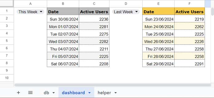
For example, based on our sample data, you can compare the number of active users this week with the number of active users last week (for the same days of the week) to observe trends.
To achieve this:
- Copy and paste the drop-down from cell A1 into cell D1.
- Use the same formula from cell B2 in cell E2, but replace
A1withD1within the formula to reference the correct drop-down. - Select “This Week” in the drop-down in cell A1 and “Last Week” in the drop-down in cell D1.
- Compare the data side by side to analyze performance trends.
This allows you to compare metrics between different weeks to observe increases, decreases, or consistency in performance over time.
Resources
- Filter Data for a Specific Number of Past Weeks in Google Sheets
- Filter or Find the Current Week This Year and Last Year in Google Sheets
- How to Filter Current Week Horizontally in Google Sheets
- Finding Week Start and End Dates in Google Sheets: Formulas
- Calculate Week Number Within Month (1-5) in Google Sheets
- Find the Date or Date Range from Week Number in Google Sheets
- Weekday Name to Weekday Number in Google Sheets
- Reset Week Number in Google Sheets Using Array or Non-Array Formulas
- Same Day Last Week Comparison in Google Sheets
- Insert Blank Rows to Separate Week Starts/Ends in Google Sheets
- Convert Dates to Week Ranges in Google Sheets (Array Formula)


