Filter Columns by Current Week in Google Sheets

Want to see only this week’s data in Google Sheets? If your columns are dated, you can filter them dynamically to show just the current week. In this guide, we’ll show you how to filter columns by current week in Google Sheets so your spreadsheet always stays up-to-date.

Whether you’re tracking employee attendance, sales, or time-based data, this method ensures you only see the relevant columns for the current week.

Table of Contents

Why Filter Columns by Current Week in Google Sheets

Filtering columns by the current week helps you:

Focus on relevant data
Reduce clutter in your spreadsheet
Automatically update as the week progresses

This technique is particularly useful for dashboards, weekly reports, and dynamic datasets.

How to Filter Columns by Current Week in Google Sheets

To filter columns by the current week, you’ll use:

FILTER function to extract the relevant columns
WEEKNUM function combined with TODAY() to determine the current week
HSTACK function to include other important columns like names or categories

Sample Dataset

Assume your spreadsheet has:

Column A: Employee names
Columns B–AF: Daily attendance or dated data
Sheet name: 'employee data'

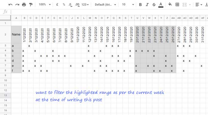
Sample Google Sheets data with employee names and daily attendance showing columns with dates as headers for filtering current week

Goal: Display only the employee names and columns where the header date falls in the current week. This view should update automatically each week.

Step 1: Filter Current Week Columns

Use this formula to filter only the columns where the date falls in the current week:

=FILTER('employee data'!B2:AF, WEEKNUM('employee data'!B2:AF2, 1)=WEEKNUM(TODAY()))

Instructions:

Paste this formula in cell A1 of a new sheet.
It will filter all columns with dates in the current week.

Tip:

WEEKNUM(..., 1) treats Sunday as the start of the week.
Use 2 instead of 1 if you want Monday as the start of the week.

Step 2: Include Employee Names with Current Week Columns

To combine the first column (employee names) with the filtered week columns, use HSTACK:

=HSTACK(
   'employee data'!A2:A, 
   FILTER('employee data'!B2:AF, WEEKNUM('employee data'!B2:AF2, 1)=WEEKNUM(TODAY()))
)

This formula creates a dynamic table showing:

Employee names
Only columns for the current week

The result updates automatically as weeks change, making it perfect for weekly reporting.

Tips for Using This Method

Ensure your header row contains valid date values.
Adjust WEEKNUM parameter according to your week-start preference.
Combine with conditional formatting to highlight current week data.

FAQs

Q1: Can I filter columns by a different week instead of the current week?
Yes. Replace TODAY() with any specific date, and WEEKNUM will calculate the corresponding week.

Q2: What if my dataset has multiple category columns?
You can include multiple columns within a single HSTACK function to combine them with the filtered data. For example:
=HSTACK('employee data'!A2:B, ...)
=HSTACK('employee data'!A2:A, 'employee data'!Z2:Z, ...)

Q3: Can this work for monthly filtering?
Yes. Instead of WEEKNUM, use MONTH() in the FILTER formula to filter by the current month.