Convert Dates to Week Ranges in Google Sheets (Array Formula)

We can employ an array formula to convert dates in a column into week ranges, whether combined or separated, within Google Sheets.

You can maintain the week ranges in two distinct columns, one for the week’s start date and another for the end date, or combine them.

However, combining has a drawback. When you employ the combined week ranges for sorting, it won’t arrange them as intended; it will sort alphabetically since it’s treated as text. Can we address this issue as well?

Absolutely. We can resolve this by prefixing sequential numbers with ’00’ text formatting code to the combined week ranges.

Important:

When converting dates to week ranges, we won’t take into account week numbers or specific days of the week. The initial week commences with the lowest date in the column, and the final week concludes with the highest date in the column—something akin to what you may have observed in an Excel Pivot Table.

If you’re interested in converting the dates to week ranges based on the week numbers, I have a separate tutorial for that. I’ll provide a link to it at the end of this post.

Converting Dates to Week Ranges: Separate Start and End Dates

To convert the dates in the range A2:A into week ranges, you can use the following array formula in any available blank cell. Afterward, select the result and apply Format > Number > Date.

=LET(
     range, A2:A, 
     n, (MAX(range)-MIN(range))/7, 
     IFNA(
          HSTACK(
               SEQUENCE(n+1, 1, MIN(range), 7), 
               IFERROR(SEQUENCE(n, 1, MIN(range)+6, 7), MAX(range))
          ), MAX(range)
     )
)

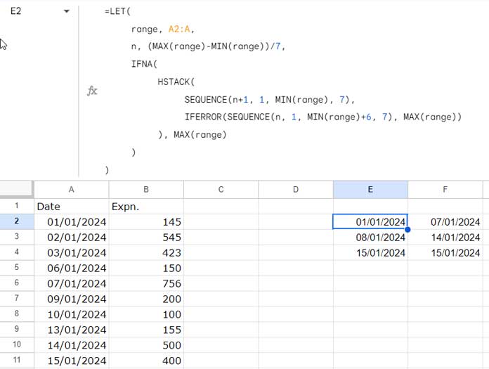
Converting dates into week ranges, displayed in two columns.

The formula returns week start dates in one column and end dates in another. Ensure there are sufficient blank cells for the formula to expand; otherwise, it will result in a #REF error.

Assigning Week Ranges to Corresponding Dates:

For instance, assuming dates are in column A (A2:A) and expenses are in column B (B2:B), the formula in cell E2 will convert the dates in A2:A to week ranges in E2:F.

Let’s associate these converted week ranges with the corresponding dates using XLOOKUP.

In cell C2, use the following formula to assign the start dates in E2:E corresponding to the dates in A2:A:

=ArrayFormula(XLOOKUP(A2:A, E2:E, E2:E,,-1))

For the end dates in F2:F, insert the following formula in cell D2:

=ArrayFormula(XLOOKUP(A2:A, E2:E, F2:F,,-1))

Select C2:D and apply Format > Number > Date.

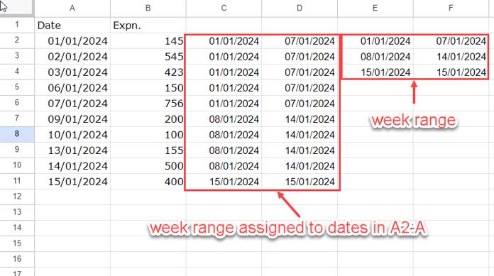
Image illustrating the assignment of week ranges into two columns.

So, we have successfully converted dates into week ranges and linked them to their corresponding dates.

Anatomy of the Formulas

Let’s start with the formula for converting dates to week ranges. Then, we’ll delve into the explanation of the XLOOKUP functions.

a. How the Formula Converts Dates to Date Ranges

The formula employs the LET function, enabling the declaration of variables for later use in the formula.

Syntax: LET(name1, value_expression1, [name2, …], [value_expression2, …], formula_expression)

Names and Value Expressions:

range, A2:A: Assigns the variable ‘range’ to the dates in A2:A, allowing later parts of the formula to refer to it.

n, (MAX(range)-MIN(range))/7: Calculates ‘n,’ representing the number of rows needed to populate the week start and end dates.

Formula Expression:

IFNA(
     HSTACK(
          SEQUENCE(n+1, 1, MIN(range), 7), 
          IFERROR(SEQUENCE(n, 1, MIN(range)+6, 7), MAX(range))
     ), MAX(range)
)

IFNA(…): Checks for #N/A errors and replaces them with a specified value, handling potential errors during the HSTACK operation.

HSTACK(…): Horizontally stacks arrays or values, appending results from the following sequences:

SEQUENCE(n+1, 1, MIN(range), 7): Generates a sequence starting from the minimum value in the range, incrementing with a step of 7. This creates the start date column during the conversion of dates to week ranges.
IFERROR(SEQUENCE(n, 1, MIN(range)+6, 7), MAX(range))): In this, the bold part, works similarly to the first sequence but starts from the minimum value in the range+6, returning the end dates, and increments with a step of 7. It returns one less row compared to the start dates column.
- MAX(range): If the dates to be converted fall within just one week (a very short period), the IFERROR section of the formula (the non-bold part) replaces the possible error in the end date by utilizing the maximum date in the range.

MAX(range): When stacking the week start and end dates, the formula may encounter a #N/A error in the last row of the end date column due to a row mismatch. This is addressed by replacing it with the maximum date in the range.

Therefore, when transforming dates into week ranges, the formula ensures an equal number of rows in the start and end date columns.

b. The Role of XLOOKUP in Assigning Dates

The first and second XLOOKUP formulas search the dates (A2:A) in the start date column (E2:E). The first formula returns the start dates (E2:E), while the second formula returns the end dates (F2:F).

If there is no match in the start date column, the formula will return the value from the start date column that is less than the search key. This ensures that the dates in column A fall within the converted week range.

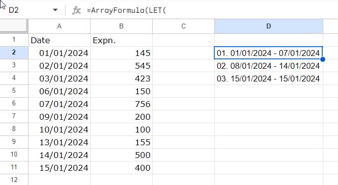
Converting Dates to Week Ranges: Combined Start and End Dates

You currently have an array formula that converts dates into week ranges, with start dates in one column and end dates in another column. However, you’re wondering how to create a true week range that combines both the start and end dates.

You can use this formula:

=ArrayFormula(LET(
     range, A2:A, 
     n, (MAX(range)-MIN(range))/7, 
     weeks, 
     IFNA(
          HSTACK(
               SEQUENCE(n+1, 1, MIN(range), 7), 
               IFERROR(SEQUENCE(n, 1, MIN(range)+6, 7), MAX(range))
          ), MAX(range)
     ), 
     formatted, 
          HSTACK(
               TEXT(SEQUENCE(ROWS(weeks)), "00."), 
               TEXT(CHOOSECOLS(weeks, 1), "DD/MM/YYY"), 
               IF(CHOOSECOLS(weeks, 1), "-",), 
               TEXT(CHOOSECOLS(weeks, 2), "DD/MM/YYY")
     ), 
     TRANSPOSE(QUERY(TRANSPOSE(formatted),, 9^9))
))

Note: Within the formula, you may replace DD/MM/YYYY with the date formatting you desire.

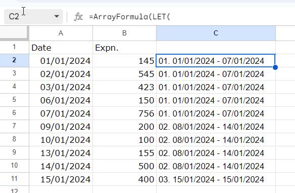
Image demonstrating the conversion of dates into combined week ranges.

However, bear in mind that direct assignment to the dates in A2:A may not be possible. Instead, you can apply this standalone formula:

=ArrayFormula(LET(
     range, A2:A, 
     n, (MAX(range)-MIN(range))/7, 
     weeks, 
          IFNA(
               HSTACK(
                    SEQUENCE(n+1, 1, MIN(range), 7), 
                    IFERROR(SEQUENCE(n, 1, MIN(range)+6, 7), MAX(range))
               ), MAX(range)
          ), 
     formatted, 
     HSTACK(
          TEXT(SEQUENCE(ROWS(weeks)), "00."), 
          TEXT(CHOOSECOLS(weeks, 1), "DD/MM/YYY"), 
          IF(CHOOSECOLS(weeks, 1), "-",), 
          TEXT(CHOOSECOLS(weeks, 2), "DD/MM/YYY")
     ), 
     weekrange, 
          TRANSPOSE(QUERY(TRANSPOSE(formatted),, 9^9)), 
     XLOOKUP(range, CHOOSECOLS(weeks, 1), weekrange, ,-1)
))

Formula Breakdown

We will start with the formula explanation of the initial formula, which transforms dates into combined week ranges, rather than delving into the second formula that assigns combined week ranges.

a. Explanation of the Formula that Generates Combined Week Ranges:

Names and Value Expressions:

range, A2:A: Assigns the variable ‘range’ to the dates in A2:A, facilitating later references within the formula.

n, (MAX(range)-MIN(range))/7: Computes ‘n,’ representing the number of rows required for week start and end date population.

weeks, IFNA(HSTACK(SEQUENCE(n+1, 1, MIN(range), 7), IFERROR(SEQUENCE(n, 1, MIN(range)+6, 7), MAX(range))), MAX(range)): Calculates ‘weeks,’ signifying the converted week range in two columns.

Up to this point, the formula adheres to our earlier method of converting dates to week ranges in two columns. The following constitute the remainder.

formatted, HSTACK(TEXT(SEQUENCE(ROWS(weeks)), "00."), TEXT(CHOOSECOLS(weeks, 1), "DD/MM/YYY"), IF(CHOOSECOLS(weeks, 1), "-",), TEXT(CHOOSECOLS(weeks, 2), "DD/MM/YYY")): Computes ‘formatted,’ essentially an HSTACK formula that stacks sequential numbers, start dates, hyphens, and end dates.

Formula Expression:

TRANSPOSE(QUERY(TRANSPOSE(formatted),, 9^9)): Utilizes QUERY to concatenate columns, combining the sequence numbers, start dates, hyphens, and end dates.

b. Explanation of the Formula that Assignes Combined Week Ranges:

This is an extended iteration of the previously explained formula that generates combined week ranges.

In this version, we’ve assigned the name ‘weekrange’ to the prior formula and incorporated the following XLOOKUP as the formula expression:

XLOOKUP(range, CHOOSECOLS(weeks, 1), weekrange, ,-1)

Where:

range corresponds to A2:A (search keys)
CHOOSECOLS(weeks, 1) refers to the start date column (lookup range)
weekrange denotes the combined week range (result range)