By converting consecutive dates into organized date ranges, we can enhance data manipulation in Google Sheets.
In this tutorial, we explore the highly effective REDUCE method that streamlines the process of summarizing consecutive dates in a column into start and end dates across two columns.
Whether you’re managing project timelines, tracking attendance, or organizing data chronologically, mastering this technique will boost your efficiency and improve the presentation of date-related information in Google Sheets.
You can effectively use functions such as ISBETWEEN within FILTER or SUMIF to aggregate data from the columns next to the date column, using the start and end dates as criteria.
Follow along step-by-step as we break down the REDUCE method to seamlessly summarize consecutive dates into usable date ranges (not text).
Sample Data and Expected Result
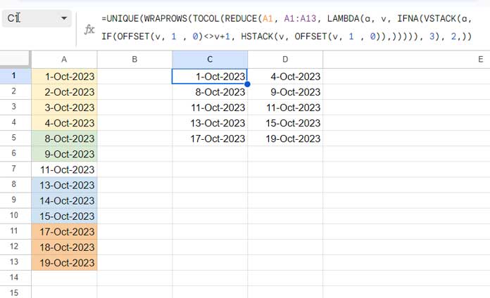
To test our REDUCE method, we will use sequential dates in column A within the range A1:A13. There will be missing sequential dates in the range.
For example, the dates in A1:A13 are as follows:
1-Oct-2023
2-Oct-2023
3-Oct-2023
4-Oct-2023
8-Oct-2023
9-Oct-2023
11-Oct-2023
13-Oct-2023
14-Oct-2023
15-Oct-2023
17-Oct-2023
18-Oct-2023
19-Oct-2023
As you can see, the sequence begins on 01-Oct-2023 and breaks on 04-Oct-2023, as the subsequent date is 08-Oct-2023. Therefore, the resulting date range should be from 01-Oct-2023 to 04-Oct-2023.
The result after applying the formula will be as follows:
| Start | End |
| 1-Oct-2023 | 4-Oct-2023 |
| 8-Oct-2023 | 9-Oct-2023 |
| 11-Oct-2023 | 11-Oct-2023 |
| 13-Oct-2023 | 15-Oct-2023 |
| 17-Oct-2023 | 19-Oct-2023 |
How do we convert consecutive dates to date ranges as shown above in Google Sheets? Let’s proceed to the formula and explanation.
Formula for Converting Consecutive Dates to Date Ranges in Google Sheets
Formula:
=UNIQUE(WRAPROWS(TOCOL(REDUCE(A1, A1:A13, LAMBDA(a, v, IFNA(VSTACK(a, IF(OFFSET(v, 1 , 0)<>v+1, HSTACK(v, OFFSET(v, 1 , 0)),))))), 3), 2,))The above formula in cell C1 will convert the consecutive dates in A1:A13 to date ranges in the cell range C1:D5.
Note: You should select the result range and apply “Format > Number > Date” to ensure that possible date values are converted to properly formatted dates.
Here are the peculiarities of the formula result:
As observed in the third row of the result, the start date and end date are the same, which is 11-Oct-2023. Why is this so?
Check the sequence in column A. The above date, i.e., 11-Oct-2023, falls between the dates 9-Oct-2023 and 13-Oct-2023. Therefore, there is no date to merge in its group.
The formula is capable of handling duplicate dates in the sequence.
The only requirement for the formula is that the dates in column A should be sorted in ascending order. If you ensure that, the formula will effectively convert sequential dates to date ranges.
Understanding How the REDUCE Formula Summarizes Consecutive Dates into Ranges
Step-by-Step Explanation:
We can separate the formula into 4 components, with the most crucial one being the REDUCE component.
REDUCE Part:
REDUCE is the core of the formula that converts the sequence of dates in column A into date ranges. Let’s break it down:
=REDUCE(A1, A1:A13, LAMBDA(a, v, IFNA(VSTACK(a, IF(OFFSET(v, 1 , 0)<>v+1, HSTACK(v, OFFSET(v, 1 , 0)),)))))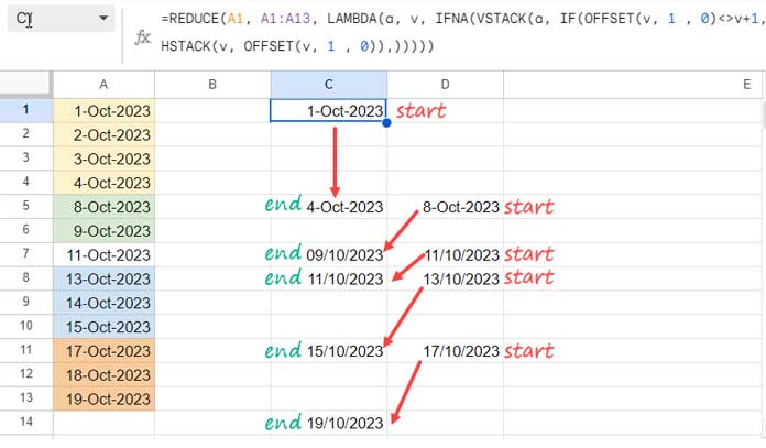
This formula iterates through the dates in A1:A13, using REDUCE to create pairs of non-consecutive dates. For each date, it checks if the next date is not consecutive (using OFFSET to compare). Here’s a closer look at the IF logical component, where v signifies the date within the current row:
IF(OFFSET(v, 1 , 0)<>v+1, HSTACK(v, OFFSET(v, 1 , 0)),)Where:
OFFSET(v, 1 , 0): next row date.v+1: current date + 1.
If the next row date is not equal to the current row date+1 (if not consecutive), it pairs the current date with the next row date using HSTACK, i.e., HSTACK(v, OFFSET(v, 1 , 0)).
The VSTACK vertically stacks the initial date in cell A1 with the result of each logical test, and IFNA handles any potential errors.
TOCOL Part:
TOCOL(…, 3)Converts the array of date pairs generated by REDUCE into a single column, arranging the dates in a start date followed by an end date format.
Additionally, the TOCOL eliminates any blank cells in between, ensuring a consolidated and structured presentation of the date ranges in the following part.
WRAPROWS Part:
WRAPROWS(…, 2)Wraps the vertical array returned by TOCOL into a two-dimensional array, with each row representing a date range.
Unique Part:
UNIQUE(…)Extracts only the unique date ranges from the array, ensuring each range appears only once.
Convert Consecutive Dates to Actionable Range Reports in Google Sheets
Presented is a real-life example that leverages date ranges derived from the REDUCE-based formula.
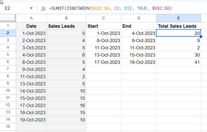
In the following example, we have dates in column A and the number of sales leads in column B.
Let’s convert the consecutive dates in the date column to date ranges and use them as criteria in SUMIF to find the total sales leads in each range.
The data starts at row #2 as row #1 contains the field labels.
Insert the following date-to-date range REDUCE formula in cell C2:
=UNIQUE(WRAPROWS(TOCOL(REDUCE(A2, A2:A, LAMBDA(a, v, IFNA(VSTACK(a, IF(OFFSET(v, 1 , 0)<>v+1, HSTACK(v, OFFSET(v, 1 , 0)),))))), 3), 2,))This formula will convert consecutive dates to date ranges in cells C2:D.
In cell E2, insert the following SUMIF formula and copy-paste down:
=SUMIF(ISBETWEEN($A$2:$A, C2, D2), TRUE, $B$2:$B)Here, the ISBETWEEN function determines which dates in $A$2:A fall between C2 and D2, returning an array of TRUE and FALSE. The SUMIF function then sums the corresponding values in $B$2:B only for those positions where ISBETWEEN returned TRUE.
Note: You can convert this formula to an array formula using the MAP Lambda function. However, since our focus is on converting sequential dates to date ranges, I won’t delve into that aspect.


