We can utilize either the comparison operators or the ISBETWEEN function to include a date range in SUMIFS in Google Sheets.
In both of these methods, you have the flexibility to use date functions, not limited to plain dates or cell references. Still confused?
You can directly input (hardcode) the date within the formula, reference specific cells, or make use of date functions like TODAY, EOMONTH, and more.
What is meant by a ‘date range’ in SUMIFS?
In simple terms, it means summing a column when the dates in another column fall between two specific dates. As mentioned earlier, there are various ways to reference these two dates within the SUMIFS function.
It’s important to note that SUMIFS is not the only function available for summing a column based on a date range. You can also consider using QUERY, SUMPRODUCT, or SUM + FILTER to achieve this.
In this tutorial, you will learn how to apply date criteria in Google Sheets SUMIFS. Take a look at the example formulas provided.
Methods to Include a Date Range in SUMIFS in Google Sheets
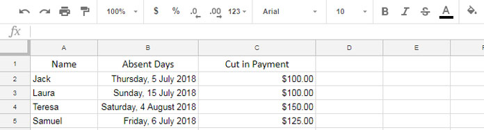
The sample data consists of employee names in column A, their absence days in column B, and the deduction in payment in column C. The data range is A1:C, but for the formulas, we will use A2:C, as A1:C1 contains field labels.
Here is the SUMIFS syntax for your quick reference:
SUMIFS(sum_range, criteria_range1, criterion1, [criteria_range2, …], [criterion2, …])In the sample data, you can use this syntax to calculate SUMIFS for a date range in Google Sheets.
Plain Dates as Date Range Criteria in SUMIFS
Learn how to calculate the sum of values in column C when the dates in column B fall between 01/07/2018 (the first criterion) and 31/07/2018 (the second criterion).
Formula:
=SUMIFS(C2:C,B2:B,">="&DATE(2018,7,1),B2:B,"<="&DATE(2018,7,31)) // returns 325You can include a date range in SUMIFS in Google Sheets using this method. In this formula, I have manually set the criteria and employed the >= and <= comparison operators.
The same formula can be written using the ISBETWEEN function instead of comparison operators:
Formula:
=SUMIFS(C2:C,ISBETWEEN(B2:B,DATE(2018,7,1),DATE(2018,7,31)),TRUE) // returns 325Here is the ISBETWEEN syntax for your quick reference:
ISBETWEEN(value_to_compare, lower_value, upper_value, [lower_value_is_inclusive], [upper_value_is_inclusive])Explore more example formulas.
Cell References as Date Range Criteria in SUMIFS
This time, I’m including a screenshot to help you understand the formula.
This SUMIFS formula would also yield the same result as above:
=SUMIFS(C2:C,B2:B,">="&D7,B2:B,"<="&E7)
=SUMIFS(C2:C,ISBETWEEN(B2:B,D7,E7),TRUE)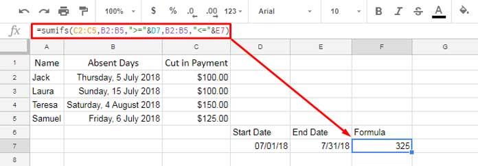
Where:
D7 contains the start date, and E7 contains the end date (the first and second criteria).
I’m providing more formula examples to further familiarize you with the usage of date criteria in SUMIFS in Google Sheets.
How to Use Date Functions in SUMIFS as Criteria
Learn how to use date functions in SUMIFS. I am incorporating two date functions here – TODAY and EOMONTH.
SUMIFS to Sum a Column Based on the Dates Falling in the Current Month
Learn how to incorporate a date range into SUMIFS in Google Sheets using various methods. The formula below is exceptionally flexible as the total automatically adjusts based on the current month.
Firstly, understand how to find the starting date of the current month in Google Sheets. It involves a clever use of the TODAY and EOMONTH combination.
=EOMONTH(TODAY(),-1)+1This formula will return the starting date of the current month in Google Sheets. To find the end date of the current month, refer to the following formula:
=EOMONTH(TODAY(),0)Now, see how to incorporate these two dynamic dates as criteria in SUMIFS.
=SUMIFS(C2:C,B2:B,">="&EOMONTH(TODAY(),-1)+1,B2:B,"<="&EOMONTH(TODAY(),0))
=SUMIFS(C2:C,ISBETWEEN(B2:B,EOMONTH(TODAY(),-1)+1,EOMONTH(TODAY(),0)),TRUE)
This formula provides a dynamic sum in Google Sheets.
Note: If you use the sample data provided above, you may get 0 (zero) due to the use of the TODAY() function in the formula. Please replace the dates in column B with the dates from the current month.
Finally, take a look at another formula where I’ve included an additional condition apart from the dates:
=SUMIFS(C2:C,A2:A,"Teresa",B2:B,">="&EOMONTH(TODAY(),-1)+1,B2:B,"<="&EOMONTH(TODAY(),0))
=SUMIFS(C2:C,A2:A,"Teresa",ISBETWEEN(B2:B,EOMONTH(TODAY(),-1)+1,EOMONTH(TODAY(),0)),TRUE)
This demonstrates how to include a date range in SUMIFS in Google Sheets, with the additional condition of filtering by “Teresa.”
More Resources:
- Using the Same Field Twice in the SUMIFS in Google Sheets.
- Using Different Criteria in the SUMIFS Function in Google Sheets.
- REGEXMATCH in SUMIFS and Multiple Criteria Columns in Google Sheets.
- SUMIFS Formula for Expanding Array Result in Google Sheets.
- How to Sumif/Sumifs Excluding Duplicates in Google Sheets.
- SUMIFS with OR Condition in Google Sheets.
- Highlight SUMIFS Rows Based on Its Total in Google Sheets.


Hello, I have read through multiple threads, watched tutorials, made necessary adjustments, but I still cannot get my Sumifs (with dates) to return anything but a zero. Can you please help?
— link removed by admin —
Hi, Tope,
Thanks for sharing an editable sheet with your query.
The issue was with the syntax. You were trying to follow the SUMIF syntax in SUMIFS. I have inserted a formula in cell H7. Please see that.
Hi,
I’ve gotten this to work, but wondering if you can help with something a bit more complicated.
On Sheet 2:
I have Column B = Timestamp (MM/DD/YYYY) (which is imported from Sheet 1)
I have Column C = a # (ie, 290, 130, 5, etc… its a # of tasks completed, which is imported from Sheet 1)
Goal: I am trying to add up the sums of rows of Column B, if it meets a specific date range (10/11/19 – 10/18/19) in Column A and have that total populate in Column D.
This is the equation I used and it works:
=sumifs(C2:C,B2:B,">="&date(2019,10,11),B2:B,"="&date(2019,10,18),B2:B,"<="&date(2019,10,25))And so forth…
Is there a way to do this without manually entering into each cell this formula + the specific date range I want manually for each week?
I can link the sheet if needed. Any help is appreciated!
Hi, Christine,
You can share your sheet with ‘only’ sample data and the result that you expect. I’ll try to solve it.
Best,
I am looking to use Sumifs to add a column with today’s entries with a set of data with date and time stamp.
Hi, Kushal,
In a date-time aka timestamp column, use the SUMIFS as below to sum a column based on today’s entries.
=ArrayFormula(sumifs(C2:C,A2:A,"Apple",int(B2:B),"="&today()))The INT function will return date from a timestamp. Since the INT is not an array function, in an Array, like B2:B, we must include the ArrayFormula.
The above SUMIFS formula sums column C if the text strings in A2:A = “Apple” and the dates in column B = today()
Awesome tutorial indeed! Thanks!
Thank you so much for your tutorials! I tried your formula and it worked for one date. But when I tried to use a date range it returns a 0 value.
When I apply the formula only for April 1st it works fine:
=sumifs(C:C;A:A;"2018-04-01";B:B;"2385481")And here’s my formula for the Date range:
=sumifs(C:C;A:A;">="&date(2018-4-1);A:A;"<="&date(2018-4-5);B:B;"2385481")My spreadsheet goes like this:
The C:C column is the Amount spend per advertising campaign.
The "2385481" is a unique campaign ID (column B:B).
The A:A column shows dates.
So I need to find out which campaign has the highest Amount spent for the date range between April 1st to April 5th.
The problem is that in column A:A I have multiple repeated dates (one date per each campaign ID), like so:
Date (A:A) / Campaign ID (B:B) / Amount spent (C:C)
2018-04-01 / 2385481 / 1603,98
2018-04-01 / 4538013 / 1580,42
2018-04-01 / 5391539 / 1585,47
2018-04-02 / 2385481 / 1627,53
2018-04-02 / 4538013 / 1460,40
2018-04-02 / 5391539 / 1736,25
Another issue is that I don't know all Campaign IDs (column B:B) for all of the campaigns listed in my spreadsheet. But when I try to select by referencing the cell (instead of typing in the exact campaign ID), it doesn't insert any value in the formula…
At first, I wanted to group dates (or group campaign IDs) to make it easier to then sort Amount spent by descending, but I have no idea how to do this 🙁
I would really appreciate your help! Thank you!
Hi, Valerie,
I think you have used the date in the wrong format in Sumifs as criteria.
Try the formula as below.
=sumifs(C:C;A:A;">="&date(2018;4;1);A:A;"<="&date(2018;4;5);B:B;"2385481")If you want to group data and sum, then use the Query function.
Group by Date:
=query(A1:C;"Select A, Sum(C) group by A order by sum(C) Desc")Group by Campaign ID:
=query(A1:C;"Select B, Sum(C) group by B order by sum(C) Desc")Group by Date and Campaign ID (it would return the data as it is since your Campaign IDs are not repeated. Once you have repeated Campain IDs, that also for the same date, you will see the difference.
=query(A1:C;"Select A,B, Sum(C) group by A,B order by sum(C) Desc")You can check my Functions Guide to learn Query.
Hello
How can you add a condition that provides the result if A2:A5 is Teresa OR Laura?
=sumifs(C2:C5,A2:A5,"Teresa",B2:B5,">="&EOMONTH(TODAY(),-1)+1,B2:B5,"<="&EOMONTH(TODAY(),0))Hi, Rocio,
You can use multiple criteria in Sumifs in the same column using Regexmatch and ArrayFormula.
=ArrayFormula(sumifs(C2:C5,regexmatch(A2:A5,"Teresa|Laura"),TRUE,B2:B5,">="&EOMONTH(TODAY(),-1)+1,B2:B5,"<="&EOMONTH(TODAY(),0)))
See my earlier tutorial related to it - REGEXMATCH in SUMIFS and Multiple Criteria Columns in Google Sheets
Thanks.
Brilliant tutorial, exactly what I needed. Thanks!