Want to visually identify the rows that are being summed by a SUMIFS formula? You can do that by combining SUMIFS with a row-wise logical comparison inside conditional formatting in Google Sheets.
This method highlights the rows that meet multiple criteria, and you can even set conditions based on the total—like whether the total is less than or greater than a target value.
In this tutorial, we’ll walk through:
- How to highlight rows that SUMIFS adds up
- How to conditionally highlight them based on the total value
Why Highlight SUMIFS Rows?
When you use a SUMIFS formula to get a total, Google Sheets won’t automatically show which rows contributed to that total. This can be frustrating—especially when editing or analyzing data.
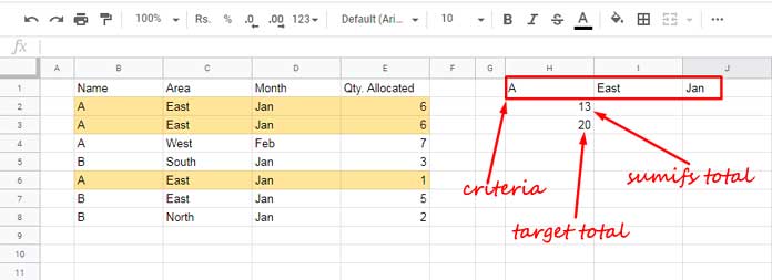
Let’s say the criteria are:
- Name = “A”
- Area = “East”
- Month = “Jan”
The SUMIFS formula might return 13, but which rows added up to 13? That’s where conditional formatting helps.
Use Case Example
Let’s say we want to highlight all rows where Name = A, Area = East, and Month = Jan. If the SUMIFS total is less than a set value—say 20—we want those rows highlighted.
This is especially useful if you’re adjusting the values in a column (like Sales or Attendance) and want to bring the total to a specific goal.
This method also helps if you’re using the Goal Seek add-on. If you try to apply Goal Seek to a row not part of the SUMIFS result, you’ll get an error like: “The goal could not be found. Subsequent iterations were not bringing the Add-on closer to a solution.”
Step 1: Logical Formula to Highlight Matching Rows
The first step is to highlight rows matching your SUMIFS criteria. We do this with a simple logical condition.
Formula:
=$B2 & $C2 & $D2 = $H$1 & $I$1 & $J$1This formula:
- Concatenates the values in each row of columns B, C, and D
- Compares them to the combined criteria in cells
H1,I1, andJ1 - Returns TRUE for matching rows, which conditional formatting can then highlight
Tip: Apply this rule to a range like B2:E to highlight full rows, or restrict it to a specific column if needed.
Step 2: Add a SUMIFS Total for Context (Optional)
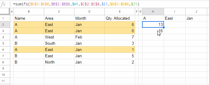
While the formula above highlights matching rows, it doesn’t check their total. For that, we add a SUMIFS formula in a helper cell.
Example:
=SUMIFS($E$2:$E, $B$2:$B, $H1, $C$2:$C, $I1, $D$2:$D, $J1)This gives you the total from column E based on the criteria.
Let’s say this total is in H2, and we want to compare it to a target in H3.
Step 3: Conditionally Highlight Based on SUMIFS Total
Now we combine everything to highlight rows only if the SUMIFS total meets your threshold.
Formula:
=IF($H$2 < $H$3, $B2 & $C2 & $D2 = $H$1 & $I$1 & $J$1)$H$2 < $H$3checks if the total is below your target- The right side ensures only the matching rows are highlighted
Want to highlight if the total is greater than the target instead? Change < to > in the formula.
Step 4: How to Apply the Highlighting Rule in Google Sheets
Follow these steps to apply the custom conditional formatting rule:
- Select the range — e.g.,
B2:Eif you want to highlight full rows. - Go to Format > Conditional formatting.
- Under Format rules, choose Custom formula is.
- Enter the formula — for example:
=IF($H$2 < $H$3, $B2 & $C2 & $D2 = $H$1 & $I$1 & $J$1)- Choose a highlight color and click Done.
That’s it! Google Sheets will highlight only those rows that match all three criteria and meet the total-based condition.
Conclusion
Use this approach when:
- You need to visually highlight the rows contributing to a SUMIFS result.
- You want to apply conditional logic (like goal tracking or editing support).
- You don’t want to use helper columns.
This technique is especially useful for datasets involving multi-criteria analysis. For simpler one-condition setups, use SUMIF in Conditional Formatting. For comparing entire category/group totals to individual targets, see: Highlight Groups When Their Total Exceeds a Target.
For a complete set of 80+ practical Conditional Formatting tutorials—covering everything from basic rules to advanced formula-driven techniques, including highlighting min/max values, duplicates, rows, and groups—explore the full hub: The Ultimate Guide to Conditional Formatting in Google Sheets — your one-stop resource for mastering all aspects of conditional formatting.


