Want to highlight rows if the SUMIF total is less than or greater than a certain value (target) in Google Sheets? Yes, it’s possible! You can use SUMIF in conditional formatting to highlight cells or rows based on whether they meet a specific threshold.
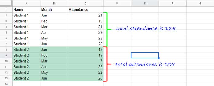
Let’s take an example: Suppose we have the total attendance of two students from 01-01-2019 to 30-06-2019. We want to check whether they meet the minimum required attendance to qualify for an exam.
Condition: A student must have at least 120 days of attendance to be eligible.
See the sample data and how we use SUMIF in conditional formatting to achieve this.
Must Read: Google Sheets Functions Guide (Quickly Learn All Popular Functions in Sheets)
How to Use the SUMIF Formula in Conditional Formatting
Here’s the mock data used in Google Sheets:
Note: In this example, the data is sorted by student name. However, the SUMIF formula works perfectly even if your data is not sorted. Sorting is not a requirement for this conditional formatting to work correctly.
We’ll use a custom SUMIF formula in conditional formatting for two different purposes:
- Highlight cells/rows when the SUMIF total meets the target
- Highlight cells/rows when the SUMIF total doesn’t meet the target
To switch between these, you just need to adjust the comparison operator in the formula.
SUMIF to Highlight Rows if Total is Less Than the Target
SUMIF Custom Formula Rule #1:
=AND($A2<>"", SUMIF($A$2:$A, $A2, $C$2:$C) < 120)This SUMIF conditional formatting formula highlights rows where the total attendance per student is less than 120. For example, it highlights the rows for “Student 2” in column A.
Note: The AND function ensures that blank rows are excluded from highlighting.
Steps to Apply:
- Select the range (e.g.,
A2:Cbased on your dataset) - Go to the Format menu → Conditional formatting
- Under Format rules, choose Custom formula is
- Enter the formula above
- Choose your formatting style
- Click Done
SUMIF to Highlight Rows if Total is Greater Than or Equal to the Target
Sometimes, you may want to highlight students who meet or exceed the attendance requirement.
SUMIF Custom Formula Rule #2:
=AND($A2<>"", SUMIF($A$2:$A, $A2, $C$2:$C) > 119)This highlights the rows for “Student 1” because the total attendance is sufficient.
Highlight Only a Specific Column Instead of Entire Rows
Want to highlight just the names in column A instead of full rows? You don’t need to change the formula — just modify the Apply to range.
Use the same formula:
=AND($A2<>"", SUMIF($A$2:$A, $A2, $C$2:$C) > 119)Then, in the conditional formatting pane, set the Apply to range to A2:A instead of A2:C.
This way, only the names in column A will be highlighted.
As you can see, it’s easy to use SUMIF in conditional formatting without needing any helper columns.
Related Use Cases
Looking for more advanced conditional formatting use cases with SUMIF or SUMIFS?
- Highlight Groups When Their Total Exceeds a Target in Google Sheets — for setting individual target totals per group or category, including support for a second lookup table.
- Highlight SUMIFS Rows Based on Its Total in Google Sheets — to highlight specific rows that match multiple conditions and check whether their total meets a given threshold.
These tutorials expand on this method with more advanced logic for grouped data or multi-criteria highlighting.
This example shows how you can combine aggregation functions with conditional formatting to create powerful, criteria-based highlights in Google Sheets. For a broader collection of techniques—from basic rules to advanced formula-driven scenarios—see: The Ultimate Guide to Conditional Formatting in Google Sheets.


Hi,
I’m trying to change the font color in cells under column M to bold and red if the sum of the cells in the row for each cell equals zero.
I’m using your formula as so:
Range: M4:M56
Custom condition:
=AND($D4="Approved",SUM($P4:$AA4)=0)What am I missing?
Hi, Joe,
Use SUM, not SUMIF. You can try …
=AND($D4="Approved",SUM($P4:$AA4)=0)Thanks, I tried that, but it didn’t work initially.
However, eventually, I figured why.
I have 6 other conditional formatting on the sheet, and this one was the last.
But when I moved to the top of the list, it worked.
I’m not sure why? But all of them seem to work properly now.
Hi, Joe,
The custom highlight rule order does matter in conditional formatting.
Hello, I’m trying to use this formula in the conditional formatting but it doesn’t work:
SUMIFS(Cobros!$D:$D;Cobros!$I:$I;$B2;Cobros!$J:$J;MONTH(U$1);Cobros!$K:$K;YEAR(U$1)-2000)) = U2
The “SUMIFS” works perfectly if I use it in another cell, but it doesn’t work in the conditional formatting. Can you help me, please?
Regards,
Guillermo
Hi, Guille,
Enter your following SUMIFS in cell U3.
=SUMIFS(Cobros!$D:$D,Cobros!$I:$I,$B$2,Cobros!$J:$J,MONTH($U$1),Cobros!$K:$K,YEAR($U$1)-2000)
Then in conditional formatting try these rules (first select entire sheet).
Rule 1:
=isblank($I1)=trueRule 2:
=and($U$2=$U$3,regexmatch(to_text(row($A1:$A)),textjoin("|",1,filter(row($A$1:$A),$I:$I=$B$2,
$J:$J=month($U$1),$K:$K-year($U$1)-2000))))
See if that works?