In Google Sheets, conditional formatting enables you to dynamically highlight entire rows based on specific criteria.

Applying the rule is straightforward when you know the column to search. For example, you might have date entries in column A and want to highlight rows where column A contains today’s date.

However, it becomes trickier when you want to search across multiple columns or match more complex conditions.

In this tutorial, you’ll learn how to highlight entire rows based on:

• A specific column
• Multiple values
• Any column in a range
• Lookup-based conditions (VLOOKUP/XLOOKUP)

Quick Answer: Highlight an Entire Row in Google Sheets

To highlight an entire row in Google Sheets using conditional formatting:

• Select your data range (e.g., A5:E100)
• Go to Format → Conditional formatting
• Choose Custom formula is
• Enter a formula like:

=$A5=TODAY()

• Click Done

Tip: Use an absolute column (e.g., $A) and a relative row (e.g., 5) to apply the rule across entire rows.

This method works for most row-highlighting scenarios using custom formulas.

Highlight Entire Rows Based on a Specific Column

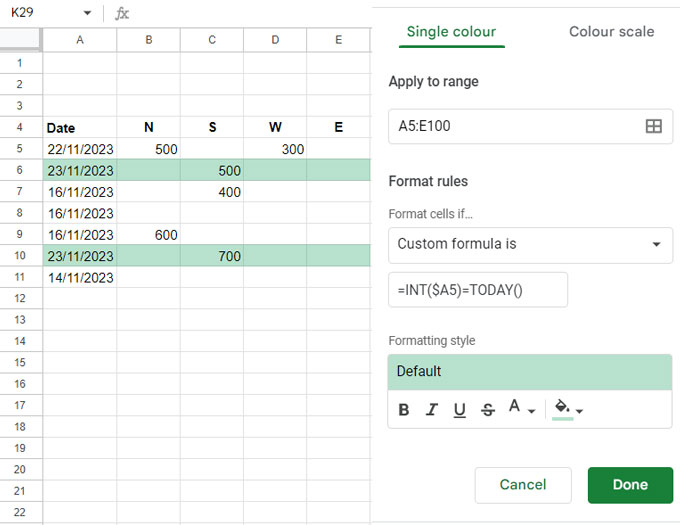
In the following example, the goal is to highlight rows in the range A5:E100 where column A contains today’s date.

Steps:

• Go to Format → Conditional formatting
• In Apply to range, enter A5:E100
• Select Custom formula is
• Enter:

=INT($A5)=TODAY()

• Choose your formatting style
• Click Done

This highlights all rows where column A contains today’s date, including timestamps.

Make sure the row reference ($A5) corresponds to the first row of your “Apply to range”. If your range starts from a different row (for example, A1:E100), update the formula accordingly:

=INT($A1)=TODAY()

Other Criteria Examples

You can modify the formula based on your requirement:

• Specific date: =INT($A1)=DATE(year, month, day)
• Text match: =$A1=”Apple”
• Number: =$A1=100
• Comparison: =$A1>=100

Highlight Rows Using Multiple Conditions (OR Logic)

To highlight rows based on multiple values, apply the rule to your data range (for example, A5:E100) and use the following custom formula:

=OR($B5="Apple", $B5="Orange")

This formula checks whether the value in column B is either “Apple” or “Orange”.
If any one of the conditions is TRUE, the entire row will be highlighted.

Tip: To learn more about combining conditions, see AND, OR, and NOT in Conditional Formatting in Google Sheets.

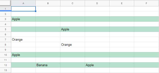
Highlight Rows Based on Values Across Multiple Columns

If you don’t know which column contains the value, use this approach.

Apply the rule to your data range (for example, A1:Z1000) and use the following custom formula:

=XMATCH("Apple", $A1:$Z1)

This formula searches across each row within the specified range. If the value “Apple” is found in any column of a row, the formula returns a match, and the entire row is highlighted.

Highlight Entire Row Using VLOOKUP

In the following example, the table is in the range A3:E11, and the goal is to highlight the entire row containing the first occurrence of the value “Blueberry” in A3:A11.

Use the following formula in Apply to range A3:E11:

=ROW()=ROW(INDIRECT(CELL("ADDRESS", VLOOKUP("Blueberry", $A$3:$E11, 2, 0))))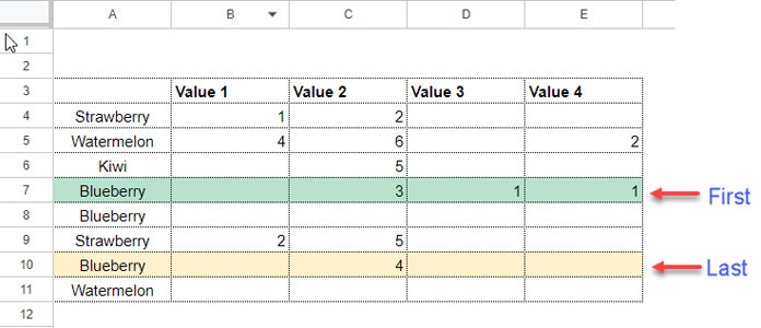

How This Formula Works

• VLOOKUP("Blueberry", $A$3:$E11, 2, 0)
  Searches for “Blueberry” in the first column of the range and returns a value from the second column.
  (The return column is not important here—any column index from 2 to 5 will work.)
• CELL("ADDRESS", …)
  Returns the cell reference (address) of the result returned by VLOOKUP
• INDIRECT(...)
  Converts the text address into a real cell reference
• ROW(...)
  Extracts the row number of that reference
• ROW()
  Returns the current row number

👉 The formula compares both row numbers and highlights the matching row.

You may also find this helpful: How to Highlight VLOOKUP Results in Google Sheets (Step-by-Step), especially when working with lookup-based formatting.

Highlight Row Based on Lookup Result Conditions

If you want to apply conditions to the lookup result:

=AND(VLOOKUP("Blueberry", $A$3:$E11, 2, 0) > 3,
ROW() = ROW(INDIRECT(CELL("ADDRESS", VLOOKUP("Blueberry", $A$3:$E11, 2, 0)))))

This formula highlights the row corresponding to the first occurrence of “Blueberry”, only if the value returned from column 2 is greater than 3.

Highlight an Entire Matching Row from the Bottom of a Table

For the same sample data, you can use the following XLOOKUP formula to highlight the row corresponding to the last occurrence of a value (searching from bottom to top).

Use this formula in Apply to range A3:E11:

=ROW()=ROW(INDIRECT(CELL("ADDRESS", XLOOKUP("Blueberry", $A$3:$A11, $A$3:$A11, , 0, -1))))

How This Works

• XLOOKUP("Blueberry", $A$3:$A11, $A$3:$A11, , 0, -1)
  Searches for “Blueberry” from bottom to top and returns the last matching value
• CELL("ADDRESS", …)
  Returns the cell address of the matched value
• INDIRECT(...)
  Converts the address text into a valid reference
• ROW(...)
  Extracts the row number of that reference
• ROW()
  Returns the current row number

👉 The formula highlights the row where both row numbers match (i.e., the last occurrence).

Limitations and Tips

• Conditional formatting works row by row, so formulas must align with row logic
• Incorrect use of $ (absolute references) is the most common mistake
• Searching across large ranges may impact performance
• Complex formulas (VLOOKUP/XLOOKUP) can be harder to maintain

When Should You Use Each Method?

• Known column → use simple $A5-based formulas
• Multiple values → use OR()
• Unknown column → use XMATCH()
• Lookup-based logic → use VLOOKUP() or XLOOKUP()

Common Mistakes When Highlighting Entire Rows

When applying conditional formatting to highlight entire rows, small mistakes in formulas or ranges can lead to incorrect results. Here are some common issues to watch for:

1. Incorrect Use of Absolute and Relative References

One of the most common mistakes is not fixing the column reference properly.

• ✔ Correct: $A5 (absolute column, relative row)
• ❌ Incorrect: A5 or $A$5

If you don’t lock the column, the formula may shift across columns and fail to highlight entire rows correctly.

2. Mismatch Between Formula and Apply to Range

Your custom formula must align with the top-left cell of the “Apply to range”.

For example:

• If the range is A5:E100, your formula should reference row 5 (e.g., $A5)
• Using $A1 here would produce incorrect results

3. Using Full Column References in Row-Based Rules

Avoid formulas like:

=A:A="Apple"

This won’t work as expected in conditional formatting for rows.

Instead, always reference the current row:

=$A5="Apple"

4. Forgetting That Rules Are Evaluated Row by Row

Conditional formatting applies the formula separately to each row.

This means:

• The formula should return TRUE/FALSE for each row
• Functions that return arrays may not behave as expected

5. Overcomplicating Simple Conditions

In many cases, a simple formula like:

=$A5="Apple"

works better than complex lookup-based formulas.

Use advanced formulas (like VLOOKUP or XLOOKUP) only when necessary.

6. Ignoring Performance on Large Ranges

Applying complex formulas (like XMATCH, VLOOKUP, or XLOOKUP) over large ranges (e.g., A1:Z1000) can slow down your sheet.

👉 Try to:

• Limit the range where possible
• Use simpler conditions when available

Tip

If your rule is not working as expected, test the formula directly in a cell first.
If it returns TRUE/FALSE correctly, it should work in conditional formatting.

Conclusion

Highlighting entire rows in Google Sheets using conditional formatting depends on how you define your condition. Whether you’re working with a single column, multiple criteria, or lookup-based logic, using the correct combination of absolute and relative references is key.

For example, $B5 ensures that the column remains fixed while the row adjusts dynamically.

For a broader understanding of conditional formatting, including rules, tips, and advanced techniques, see The Ultimate Guide to Conditional Formatting in Google Sheets.

Additional Resources

• How to Highlight an Entire Column in Google Sheets – Apply conditional formatting to columns instead of rows