Quick Answer
To highlight VLOOKUP results in Google Sheets, use the following custom conditional formatting formula:
=ADDRESS(ROW(), COLUMN())=CELL("address", VLOOKUP($E$1, $A$2:$C$6, $E$2, FALSE))This works because, in Google Sheets, VLOOKUP can return a reference to the matched cell, allowing CELL to extract its address and compare it with each cell in the selected range.
Introduction
Unlike Excel, Google Sheets can return a cell reference from VLOOKUP (when the index column is not 1). This allows us to highlight the exact lookup result by matching each cell’s address with the VLOOKUP result.
However, there is one limitation:
- If the index column is 1, this method won’t work
- In such cases, you typically don’t need VLOOKUP, as you are already referencing the lookup column. Instead, you can use a simple condition like
=B2=$E$1in conditional formatting.
Examples to Highlight VLOOKUP Results in Google Sheets
You can use VLOOKUP to:
- Highlight exact matches in sorted or unsorted data
- Highlight the exact match or next smaller value in sorted data
Highlight Exact Match in VLOOKUP
Assume you have the following data in A1:C6:
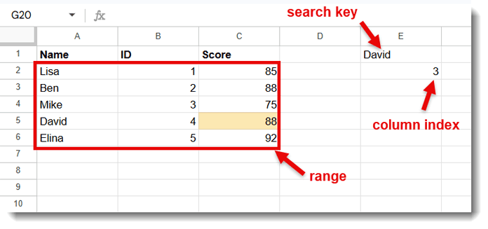
- Search key → E1 (e.g., David)
- Column index → E2 (e.g., 3 for Score)
Formula
=ADDRESS(ROW(), COLUMN())=CELL("address", VLOOKUP($E$1, $A$2:$C$6, $E$2, FALSE))👉 This will highlight cell C5 (David’s score).
- To highlight the ID instead, change E2 to 2
- Changing the name in E1 updates the highlight automatically
How to Apply the Rule
- Select the range A2:C6 (exclude header row)
- Go to Format > Conditional formatting
- Choose Custom formula is
- Enter the formula
- Choose a formatting style
- Click Done
How This Formula Works
VLOOKUPreturns the matched valueCELL("address", …)returns the cell address of that valueADDRESS(ROW(), COLUMN())returns the current cell address
👉 The formula compares both addresses and highlights the matching cell.
Highlight Exact Match or Next Smaller Value (Sorted Data)
In a sorted dataset, you can highlight either:
- Exact match
- Or the next smaller value
Example
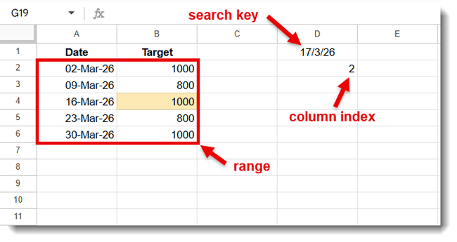
- Data range → A1:B6
- Apply to range → A2:B6
- Search key → D1
- Column index → D2
Formula
=ADDRESS(ROW(), COLUMN())=CELL("address", VLOOKUP($D$1, $A$2:$B$6, $D$2, TRUE))👉 If D1 contains a date between 16-Mar-26 and 22-Mar-26, it will highlight B4.
Important Notes
- This method works only when the VLOOKUP range is a direct (physical) range reference.
- Ensure your lookup range and column index are correct.
- The column index should not be 1, as the formula relies on retrieving a reference from a different column.
Conclusion
In this tutorial, we explored the easiest way to highlight VLOOKUP results in Google Sheets using conditional formatting.
This method allows you to dynamically track lookup results and make your data more interactive and visually clear.
If you want to reference data from another sheet, you can use INDIRECT within the VLOOKUP formula.
This tutorial is part of The Ultimate Guide to Conditional Formatting in Google Sheets, where you can explore 80+ practical examples, including lookup-based highlighting, dynamic rules, and advanced formatting techniques.


