Do you want to search a row and column for specific values and highlight their intersections in Google Sheets? This is a common task when working with two-way lookup tables, and you can achieve it using a simple conditional formatting formula.
Use the following formula to highlight the intersection in Google Sheets:
=ADDRESS(ROW(), COLUMN())=CELL("address", XLOOKUP(searchKey_v, first_col, XLOOKUP(searchKey_h, first_row, table)))searchKey_v→ the value to look up in the first column (row lookup)searchKey_h→ the value to look up in the first row (column lookup)first_col→ the range of the first column in your tablefirst_row→ the range of the first row in your tabletable→ the full table range
⚠️ When using cell or range references, make sure they are absolute references (with $) to avoid errors in conditional formatting.
Understanding Intersection Values in a Two-Way Lookup
Before highlighting intersections, it’s essential to understand what an intersection value is.
Imagine you have the following table in the range B2:E6:
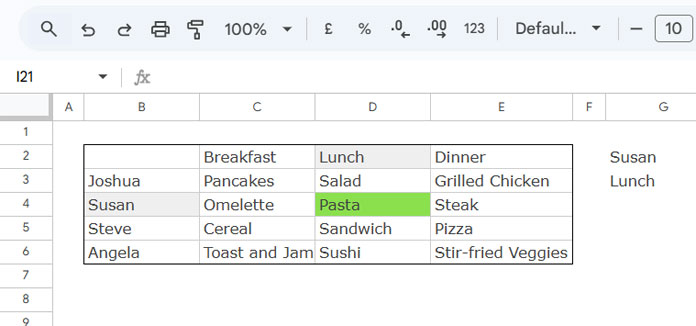
If you want to highlight Susan’s lunch, you’ll need to:
- Look up “Susan” in the first column.
- Look up “Lunch” in the first row.
The value at the intersection is “Pasta”, which we want to highlight.
Step-by-Step: Highlight Intersections in Google Sheets
Follow these steps to highlight the intersection value:
- Enter the search keys:
G2→ SusanG3→ Lunch
- Select the table range:
B2:E6. - Go to Format → Conditional Formatting.
- In the sidebar under Single Color, select Custom formula is.
- Enter the following formula:
=ADDRESS(ROW(), COLUMN())=CELL("address", XLOOKUP($G$2, $B$2:$B$6, XLOOKUP($G$3, $B$2:$E$2, $B$2:$E$6)))
- Choose a formatting style (e.g., fill color, text color).
- Click Done.
✅ Now, the cell containing Susan’s lunch preference (“Pasta”) will be highlighted automatically.
Adapting the Formula for a Different Table
To adjust this formula for another range:
- Replace
$G$2with the cell containing your row lookup value. - Replace
$G$3with the cell containing your column lookup value. - Update the ranges:
$B$2:$B$6→ first column of the table$B$2:$E$2→ first row of the table$B$2:$E$6→ full table range
Keep absolute references ($) to ensure conditional formatting works correctly.
How the Formula Works
The formula uses nested XLOOKUP:
XLOOKUP($G$2, $B$2:$B$6, XLOOKUP($G$3, $B$2:$E$2, $B$2:$E$6))
- Inner XLOOKUP: Finds the column for the selected header (
Breakfast,Lunch,Dinner). - Outer XLOOKUP: Finds the row for the selected name (
Susan). - CELL(“address”, …): Returns the actual cell address of the intersection.
- ADDRESS(ROW(), COLUMN()): Checks if the current cell matches the intersection.
When matched, the conditional formatting highlights the cell.
Conclusion
You can use this approach to highlight two-way lookup results dynamically in Google Sheets.
This technique is part of the hub post: The Ultimate Guide to Conditional Formatting in Google Sheets, which contains a comprehensive collection of tips and examples to visually analyze your data.


V E R Y clever! And really useful. Thanks!