The two-way filter in Google Sheets – What does it mean?
Two-way filter formula extracts rows and columns that meet the given criteria/conditions. I think we can call it a dynamic horizontal and vertical filter in Google Sheets.
I have not seen any tutorial or tips related to two-way filtering in Google Sheets or Excel so far.
So most probably you are also new to this two-way filter concept. But I have only the formula for Google Sheets users.
Just like two-way lookup, a two-way filter is also possible in Google Sheets.
Must Check: How to Perform Two-way Lookup Using Vlookup in Google Sheets.
In this new iteration of Google Sheets tutorial, I am providing you the said filter formula. Just follow my tips to modify the formula to match your data range and filter conditions.
To filter rows, you can either use the function Filter or Query. To filter the columns there is no any specific function.
But as a workaround, you can first transpose your data using the TRANSPOSE function and then use Query to filter rows. No doubt, that would be equal to filtering columns.
In two-way filtering in Google Sheets, I am using the functions MATCH and Query to conditionally filter rows and columns that also in a single combination formula.
Learn here all about my two-way dynamic vertical and horizontal filtering in Google Doc Sheets.
Two-way Filter in Google Sheets

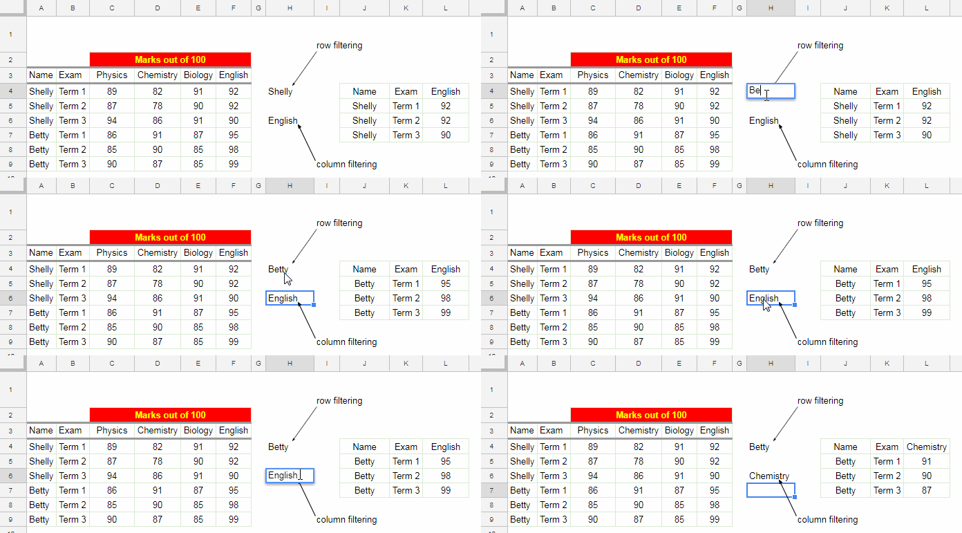
In the above example of the two-way filter in Google Sheets, I am filtering rows that contain the name “Betty” in the range A3: A (row filter) and the subject “Chemistry” in the range A3: F3 (column filter).
The Formula is in Cell J4:
=query({$A$3:$F},"Select Col1,Col2,Col"&match($H$6,$A$3:$F$3,0)&" where Col1='"&H4&"'")
How to use this formula?
{$A$3:$F} – Data range.
Select Col1, Col2, – two static columns contain Name (column A ) and Exam (column B)
For example, see this modified formula with one static column and output.
=query({$A$3:$F},"Select Col1,Col"&match($H$6,$A$3:$F$3,0)&" where Col1='"&H4&"'")
Output:

In the above example formula, I have used only one condition each in row filtering and column filtering.
The cell H6 contains the criterion to filter the columns and the cell H4 contains the criterion to filter the rows.
Let’s see how to add more criteria in the above formula that does the two-way filter in Google Sheets.
Two-way Filter in Google Sheets – Two Conditions in Row Filtering
In this new example, I am expanding the data range with one more column. See the screenshot below.
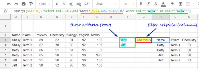
Now in my new two-way vertical and horizontal filter formula, I am applying two conditions in row filtering and one condition in column filtering.
Formula:
=query({$A$2:$G},"Select Col1,Col2,Col"&match($J$3,$A$2:$G$2,0)&" where Col1='"&I3&"' or Col1='"&I4&"'")
Output:

In this sample data, there is one new column in the data range that is column G with the marks of the students in the subject “Maths”.
Accordingly, the Query data range in the formula extended to G (A2: G). Also, the data range in the MATCH function also got modified to include the new column (A2: G2).
To include an additional filter criterion in the row, I have used the OR operator in Query which is underlined in Green color in the formula bar above.
How to Filter Columns?
If you know Query, it’s pretty easy to filter rows based on two-or-more conditions. But filtering columns are not that much easy.
Two-way Filter in Google Sheets – Two or More Conditions in Column Filtering
Use the below technique in a two-way filter in Google Sheets to filter two or more columns.
As you can see in my earlier formula, to conditionally filter only one column, I’ve used the below MATCH formula in Query.
&match($J$3,$A$2:$G$2,0)&
In this, cell J3 contains the criterion and A2: G2 is the range.
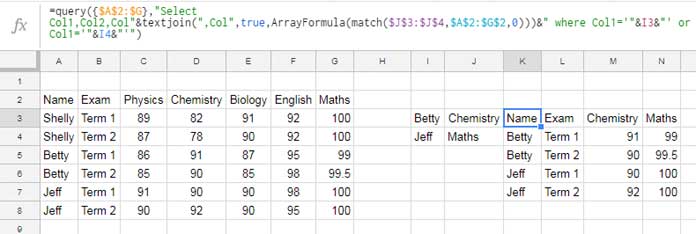
Now in my new data range, I have the criteria to filter columns in cell J3 and J4. The MATCH formula would be as follows.
&textjoin(",Col",true,ArrayFormula(match($J$3:$J$4,$A$2:$G$2,0)))&
This formula contains two additional functions. They are TEXTJOIN and ArrayFormula.
Here is the two-way or you can say horizontal and vertical filter formula and the output.
Formula:
=query({$A$2:$G},"Select Col1,Col2,Col"&textjoin(",Col",true,ArrayFormula(match($J$3:$J$4,$A$2:$G$2,0)))&" where Col1='"&I3&"' or Col1='"&I4&"'")
Output:

Now it’s easy to add additional filter columns. To add more columns, just change the MATCH function search key range as below.
&textjoin(",Col",true,ArrayFormula(match($J$3:$J$5,$A$2:$G$2,0)))&
Earlier it was J3: J4. Now I have changed it to J3: J5 to include three columns in filtering.
I think, before winding up this tutorial, I should include the screenshot of the last modification.

Hope you could understand what is the two-way filter and how to filter horizontally and vertically using a single formula in Google Sheets.
Thanks for the stay. Enjoy!


