In a three-way lookup, there are three search keys—two from separate columns and one from a row. To perform a three-way lookup in Google Sheets, I’m using only VLOOKUP and MATCH functions. Additionally, using the ampersand (&) operator or the CONCATENATE function is essential.

As a bonus, I’ll also provide a three-way lookup array formula.

If I were to use INDEX-MATCH, the popular three-way lookup method among Excel users, I wouldn’t be able to generate an array-based three-way lookup.

Let’s get started!

Example: General Ledger (GL) Data

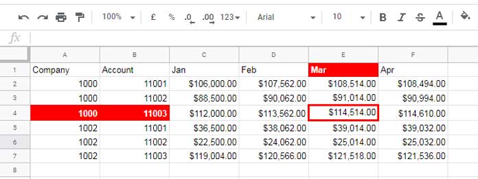
We’ll use a mock General Ledger (GL) data of a company for this demonstration.

Performing a Three-Way Lookup in Google Sheets

We need to look up:

• Company: “1000” (Column A)
• Account: “11003” (Column B)
• Month: “Mar” (Row 1)

The expected result is $114,514.00, found in cell E4.

Non-Array Formula for Three-Way Lookup in Google Sheets

First, let me show you the three-way lookup formula in Google Sheets that doesn’t automatically expand across multiple rows or columns:

=ArrayFormula(VLOOKUP(1000&11003, {A1:A&B1:B, C1:F}, MATCH("Mar", A1:F1, 0)-1, 0))

This formula is similar to a two-way lookup, but here, we’re combining two search keys using ampersand (&) to create a unique lookup value.

Explanation of the Three-Way Lookup Formula

Understanding VLOOKUP in Google Sheets can help you think differently about how to use it effectively.

• VLOOKUP typically searches for a key in the first column of a range, but we can modify this behavior.
• In our GL data (A1:F), the first search key (1000) is in Column A, and the second search key (11003) is in Column B.
• We combine the two search keys (1000&11003) and also combine Columns A and B in our data.

Thus, we transform our lookup range into:

{A1:A&B1:B, C1:F}

The third search key, “Mar,” represents the column lookup. To determine its position dynamically, we use:

MATCH("Mar",A1:F1,0)-1

This formula returns 4, meaning Column E (the March data) is the fourth column in our virtual range. The “-1” accounts for our modified column structure.

This is the easiest way to perform a three-way lookup in Google Sheets!

Array Formula for Three-Way Lookup in Google Sheets

If you need the three-way lookup to return multiple row results, understanding the non-array formula above makes this part simple.

Here’s the array formula version:

=ArrayFormula(VLOOKUP({1000&11003; 1002&11002}, {A1:A&B1:B, C1:F}, MATCH("Mar", A1:F1, 0)-1, 0))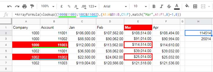

Key Differences Between the Non-Array and Array Formula:

• Instead of a single lookup value, this formula takes multiple lookup values ({1000&11003; 1002&11002}), allowing multiple results.
• The rest of the formula remains the same, ensuring it works dynamically.

Using Cell References for a Three-Way Lookup

Instead of hardcoding values, you can reference cells dynamically:

=ArrayFormula(VLOOKUP(H2:H3&I2:I3, {A1:A&B1:B, C1:F}, MATCH(J1, A1:F1, 0)-1, 0))

In this case:

• H2:H3 contains the Company values.
• I2:I3 contains the Account values.
• J1 contains the Month value.

This makes the formula more flexible and user-friendly.

Conclusion

You’ve now learned three approaches to performing a three-way lookup in Google Sheets:

1. Non-Array Formula – Useful for looking up a single value.
2. Array Formula – Expands results across multiple rows.
3. Dynamic Formula Using Cell References – More flexible and practical.

This method is particularly useful when working with financial data, inventory tracking, or any dataset with multiple search criteria.

Would love to hear your thoughts on this approach—let me know in the comments!

More VLOOKUP Resources

• VLOOKUP from Bottom to Top in Google Sheets
• VLOOKUP Result Plus Next ‘n’ Rows in Google Sheets
• Create Hyperlink to VLOOKUP Output Cell in Google Sheets
• How to VLOOKUP a Date Range in Google Sheets
• VLOOKUP Skips Hidden Rows in Google Sheets – Formula Example