Here is my attempt to compare VLOOKUP in Excel versus VLOOKUP in Google Sheets. Surprisingly, I haven’t come across any such comparison yet.
I believe both Excel and Google Sheets users could benefit from this, particularly if they’re considering switching between the two applications.
Approach this tutorial as a VLOOKUP formula comparison from the perspective of a Google Sheets expert, rather than an Excel MVP.
Given my familiarity with the VLOOKUP function in Google Sheets, my aim with this comparison is straightforward.
I’ve extensively explored various VLOOKUP formula variations in Google Sheets, all of which are available on this blog. You can easily find them by searching the site. In this comparison, I’ve attempted to replicate some of the most crucial VLOOKUP variations in Excel.
Initially, I had a general understanding of where the VLOOKUP formula might differ between Excel and Google Sheets, particularly concerning array formulas. The usage of array formulas varies between the two applications.
Make sure to check out my previous post on the differences in array formulas between Google Sheets and Excel.
Let’s start by exploring how to use VLOOKUP in Excel, and then we can delve into the comparison.
Sample Data for VLOOKUP Comparison
I’m using the following method to generate realistic sample data for the test: I’ll import a table containing FIFA World Cup finals from the provided wiki page into Google Sheets and then copy-paste it into Excel.
Use the following link in cell A1 of Google Sheets:
https://en.wikipedia.org/wiki/List_of_FIFA_World_Cup_finals
In cell B1, enter the number 5. This corresponds to the table number we’re importing from the aforementioned page for testing purposes.
Then, apply the following IMPORTHTML formula in cell A3 of Google Sheets:
=IMPORTHTML(A1, "table", B1)Google Sheets will instantly import the required table, which contains Team, Winners, Runners-up, and Total Finals into cells A3:D.
If not, it may indicate that the source has been modified. In such a case, manually enter the data as per the screenshot below. Copy the table to Excel within the same data range, i.e., A3:F16.

Note: In cell B1, the number should be 5, not 4, as the source has been modified. Although the provided screenshot reflects 4, the correct number is 5.
How to Use VLOOKUP Formula in Excel
The purpose of using VLOOKUP in Excel/Google Sheets is to search down a value in the first column of a table and retrieve a value from another column in the found row.
Below, I’m providing the basic usage. Further variations can be found in the comparison section below.
In its basic form, there’s no difference in the usage of VLOOKUP between Excel and Google Sheets.
Syntax
VLOOKUP(lookup_value, table_array, col_index_num, [range_lookup])Excel VLOOKUP Arguments (Don’t Skip this Section)
lookup_value: The value to search down in the first column of a table/dataset.table_array: The table/dataset from which to search and retrieve a value.col_index_num: The column number in the table from which to retrieve a value.range_lookup: TRUE/FALSE. Enter TRUE or 1 if the table is sorted; otherwise, enter FALSE or 0. The default is FALSE, which I’m using throughout this tutorial. This means I’m using an unsorted table for comparison purposes.
Example VLOOKUP Formula in Excel
Formula:
=VLOOKUP(E1, A4:F16, 5, FALSE)Please refer to the screenshot below.

Explanation of the VLOOKUP Formula in Excel:
In this formula, the country name “Spain” is the lookup value (located in cell E1), which should be found in the first column of the table.
Note: By default, VLOOKUP in Excel/Google Sheets only searches down the first column of the table for the search value.
The table or dataset is located in the range A4:F16. The column index to retrieve the value is 5, meaning it’s retrieved from the 5th column.
Since the data is not sorted, I’ve used the FALSE parameter, indicating that the table is not sorted. The VLOOKUP Excel formula retrieves the value from cell E11.
In a sorted range, you can specify TRUE if you want to allow an approximate match.
You can use the same VLOOKUP formula in Google Sheets without any differences.
Comparison of VLOOKUP Formula in Excel and Google Sheets
I’ve detailed the syntax of the VLOOKUP function in Excel. You can follow the same syntax in Google Sheets as well.
Let’s explore where the VLOOKUP formula in Excel and Google Sheets differs.
Handling Multiple Search Values in the Same Column with VLOOKUP in Excel and Google Sheets
As mentioned earlier, the array formula behaves differently in Sheets and Excel, which naturally impacts VLOOKUP as well.
In the example provided above, only one search value was used. Here’s how you can handle multiple search values in the same first column.
Google Sheets: VLOOKUP with Two Search Values in the Same Column
The search values are located in H2:H3, representing “Italy” and “France.”
Formula:
=ArrayFormula(VLOOKUP(H3:H4, A4:F16, 2, FALSE))Since there are two search values (lookup values), the formula is wrapped with the ArrayFormula function.
Result:

This formula extracts values from index column 2, determining how many times Italy and France won the World Cup final.
Excel: VLOOKUP with Two Search Values in the Same Column
Here’s where the Excel VLOOKUP formula differs. In Excel, there’s no need to use the ArrayFormula function since it doesn’t exist. Instead, you can directly input the VLOOKUP formula in Excel 2021 or Excel in Microsoft 365 without the need for an array formula:
=VLOOKUP(H3:H4, A4:F16, 2, FALSE)For other versions of Excel that don’t support dynamic array formulas, you’ll need to follow the legacy array formula approach using CSE (Control + Shift + Enter). Here’s how:
- Select the entire output range, here cells I3 and I4.
- Enter the above VLOOKUP formula in cell I3.
- Confirm the formula with Ctrl+Shift+Enter.
This action converts the regular VLOOKUP formula into an array formula in Excel.
The Difference in the Use of Multiple Index Columns in VLOOKUP in Excel and Google Sheets
Let’s explore how to compare VLOOKUP formulas in Excel and Google Sheets when there are multiple index columns.
Here again, the use of array functionality comes into play, resulting in differences in the formula between Excel and Google Sheets.
Here, I am going to use two index columns in VLOOKUP to retrieve values from columns 2 and 3.
Two Index Columns in VLOOKUP in Google Sheets
Formula:
=ArrayFormula(VLOOKUP(H3, A4:F16, {2, 3}, FALSE))Result:

In Google Sheets, when there are multiple index columns in VLOOKUP, they are comma-separated and wrapped by curly brackets, although alternative methods using COLUMN or SEQUENCE functions are also available.
Also, since the formula populates an array result, the entire VLOOKUP formula should be wrapped within the ArrayFormula function.
Let’s compare this Google Sheets formula with the Excel VLOOKUP formula.
Two Index Columns in VLOOKUP in Excel
CSE formula:
In Excel, first select the cells I3:J3 (result range), then enter the following formula.
=VLOOKUP(H3, A4:F16, {2,3}, FALSE)Make it an array formula by pressing Ctrl+Shift+Enter. That’s all you need to do.
Dynamic Array Formula:
Simply input this formula in cell I3. The formula will automatically spill to J3.
Comparison of VLOOKUP with Multiple Search Values and Index Columns in Google Sheets and Excel
In this case, I find Google Sheets’ VLOOKUP to be more convenient. As I mentioned earlier, approach this tutorial from the perspective of a Google Sheets expert. If you disagree with any point in this tutorial, feel free to challenge it!
From the formulas below, you can understand how VLOOKUP in Excel and Google Sheets handles two search keys and two index columns in a single formula.
Google Sheets VLOOKUP with Two Search Keys and Two Index Columns
Formula:
=ArrayFormula(VLOOKUP(H3:H4, A4:F16, {2,3}, FALSE))Simply enter this VLOOKUP array formula in cell I3, and the formula will take care of the rest.

It returns the values from the “Wins” and “Runners-up” columns (columns 2 and 3). The search keys are “Italy” and “France,” meaning there are two search keys and two index columns.
Excel VLOOKUP with Two Search Keys and Two Index Columns
In Excel, I couldn’t find a simpler way to search for two search keys and retrieve values from two columns. Follow this approach in Excel:
Select cells I3:J3 and enter the formula (remember to make it an array formula by pressing Ctrl+Shift+Enter).
=VLOOKUP(H3, $A$4:$F$16, {2,3}, FALSE)Note: If your Excel supports dynamic arrays, simply enter the formula in cell I3.
Here, two index columns are used, but only one search key. So you’ll need to copy and paste the formula down. To do that, select cells I3:J3, and drag the J3 fill handle down in the legacy array formula method, and just drag the I3 fill handle down in the dynamic array formula method.
I’ll be using a new dataset for the next comparison of VLOOKUP formulas in Excel and Google Sheets. Here it is:
VLOOKUP in Excel and Google Sheets with Search Values in Two Columns
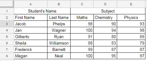
In this scenario, the first column contains students’ first names, and the second column contains their last names. Therefore, the formula needs to search down both the first and second columns.
The reason for using two search values is that the student names consist of both first and last names. Let me demonstrate how to use multiple search values in VLOOKUP in both Sheets and Excel.
Finding the mark scored by “Jan Wagner” in Chemistry – Google Sheets Approach
The ArrayFormula function in Google Sheets is more versatile than the curly bracket approach in Excel. Consequently, you can avoid using helper columns in many formulas in Google Sheets, and VLOOKUP is no exception.
In the example below, “Jan Wagner” is the search value, which spans two columns.
Formula:
=ArrayFormula(VLOOKUP(G3&H3, {A3:A8&B3:B8, C3:E8}, 3, FALSE))")
Formula Breakdown:
The first search value “Jan” is in cell G3, and the second one “Wagner” is in cell H3. Combine them in the formula using the ampersand sign.
Join the corresponding columns in the dataset as well. Although there are a total of 5 columns in the sample data, due to the concatenation of columns A and B, it’s reduced to 4. Accordingly, use the column index in VLOOKUP.
The Excel VLOOKUP Approach (Search Values in Two Columns)
The above approach won’t work with legacy array formulas (CSE) in Excel, but it does work with dynamic array formulas. Let’s start with the dynamic array formula.
Dynamic Array Formula:
=VLOOKUP(G3&H3, HSTACK(A3:A8&B3:B8, C3:E8), 3, FALSE)Here, we’ve utilized HSTACK to horizontally append two ranges: the first range is A3:A8&B3:B8 (combined first and last names), and the second range is C3:E8 (the other columns in the source table).
CSE Approach:
In this method, when there are search values in two different columns, you’ll need to utilize a helper column.
Insert a new column and designate it as the helper. Here, column C serves as the helper column.
")
In cell C3, enter the following formula and drag it down to combine the first and last names:
=A3&B3For the VLOOKUP function, the table range is C3:F8. Combine the search keys within the formula as before and input the formula as an array formula using the Ctrl+Shift+Enter shortcut.
=VLOOKUP(H3&I3, C3:F8, 3, FALSE)I am not a big fan of helper columns, so I don’t prefer this approach.
Finally, here is the comparison of VLOOKUP formulas in Excel and Google Sheets when the search key is not in the first column. This scenario is famously known as “Reverse VLOOKUP” in Excel and Google Sheets.
The Difference in Reverse VLOOKUP in Google Sheets and Excel
Due to the versatility of the ArrayFormula, in Google Sheets, it’s easy to customize the VLOOKUP in various ways, including reverse VLOOKUP.
To perform a reverse VLOOKUP, Excel requires the CHOOSE function, but Google Sheets doesn’t. Let’s see how to do it.
Find Sheila’s Marks in Maths Using Reverse VLOOKUP in Excel
In this demo data, the search value, which is the name of the student, is in the last column of the table. Please refer to the screenshot below.

VLOOKUP only supports the search value range in the first column. So, what can be done?
You can use the CHOOSE function in Excel to create a two-column virtual range where the first column contains the student’s name (D2:D8) and the second column contains the marks of the students in Maths (A2:A8).
Formula:
=VLOOKUP(F3, CHOOSE({1,2}, D3:D8, A3:A8), 2, FALSE)Enter this formula using Ctrl+Shift+Enter for legacy array formula (CSE) in Excel, and simply enter it for Excel versions that support dynamic array formulas.
Can we use this VLOOKUP + CHOOSE Excel combination formula in Google Sheets?
No, we cannot. The Google Sheets CHOOSE function is not similar to Excel’s CHOOSE. Excel’s CHOOSE function is better than the CHOOSE function in Google Sheets. I haven’t tested it in detail though.
Reverse VLOOKUP to Find Jacob’s Marks in Maths (Google Sheets Way)
Here, there is no need to use the CHOOSE function.
Formula:
=VLOOKUP(F3, {D3:D8, A3:A8}, 2, FALSE)In this formula, the search value is in cell F3. Instead of using the CHOOSE function, we can create a virtual range using curly brackets. Just shuffle the columns within the curly brackets to move the search range to the first position.


