The CHOOSE function is a basic lookup function available in both Excel and Google Sheets. In Excel, it offers an additional capability that is utilized in advanced lookups. However, Google Sheets doesn’t require this feature as it provides simple alternatives.
I’ll illustrate this difference in the CHOOSE function between Excel and Google Sheets with an example. But first, let me provide you with the syntax of the function and its general usage.
Syntax Comparison
Excel:
=CHOOSE(index_num, value1, [value2], ...)Google Sheets:
=CHOOSE(index, choice1, [choice2, ...])Let’s analyze the parameters in these functions to identify the distinctions.
In Excel, the function utilizes the parameter index_num to determine the position of the returned value, while in Google Sheets, it simply refers to this parameter as index.
Both versions of the CHOOSE function allow selecting from a list of values, but there’s a distinction in the maximum number of values that can be used. It ranges from 1 to 254 in Excel, whereas it’s limited to 1 to 29 in Google Sheets.
Additionally, the parameters for the values to choose from are labeled differently in Excel and Google Sheets: as value1, value2, … in Excel, whereas they are labeled as choice1, choice2, … in Google Sheets.
Before we proceed to learn the differences in usage of the CHOOSE function, let’s examine their basic use cases in both Google Sheets and Excel.
CHOOSE Function Basic Example in Excel and Google Sheets
Example 1:
The following CHOOSE formula will work in both Excel and Google Sheets:
=CHOOSE(2, "Sunday", "Monday", "Tuesday", "Wednesday", "Thursday", "Friday", "Saturday")It will return “Monday” since the index number is 2, and Monday is the second value (choice2).
Example 2:
The following CHOOSE formula will function well in both Excel and Google Sheets:
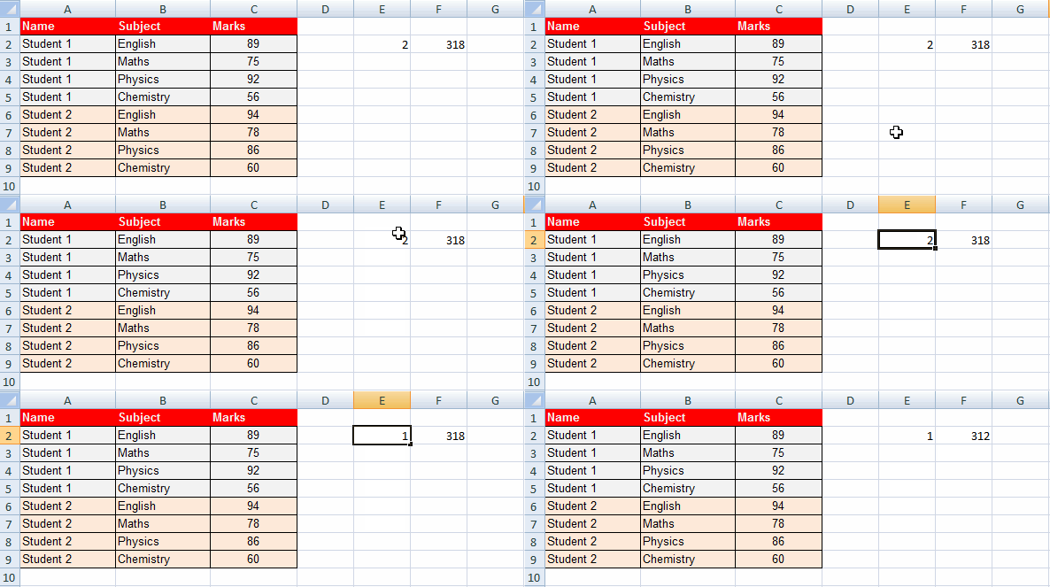
=SUM(CHOOSE(E2, C2:C5, C6:C9))In this formula, it sums either C2:C5 or C6:C9 based on the index number 1 or 2 entered in cell E2.

For more examples, you can refer to my guide on Google Sheets: “How to Use the CHOOSE Function in Google Sheets: Purpose and Examples.”
Now, it’s time to explore their difference.
How the CHOOSE Function Differs in Excel and Google Sheets
In Excel’s CHOOSE function, you can specify multiple index numbers, whereas in Google Sheets, you cannot. This is the key difference between the two.
However, this disparity doesn’t significantly affect Google Sheets’ functionality, as it has its own method to address this ‘limitation’.
Let’s examine how this feature works in Excel and the alternative approach in Google Sheets.
Formula:
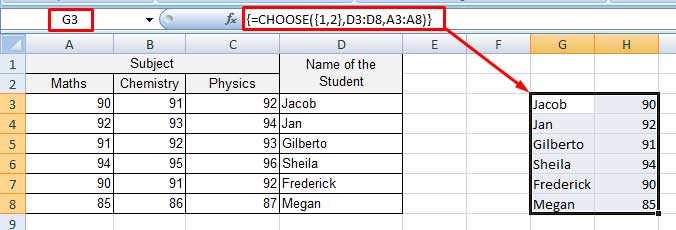
=CHOOSE({1, 2}, D3:D8, A3:A8)Let’s explore how to input/use this formula in Excel.

If you’re not using Excel 365 or Excel 2021, you should input this formula as an array formula (Ctrl+Shift+Enter). Here’s how to use the Ctrl+Shift+Enter (CSE) legacy array formula method:
Highlight the cell range G3:H8 (result range) and enter the formula in cell G3. Then press Ctrl+Shift+Enter.
In Excel versions supporting dynamic array formulas, you only need to input this formula in cell G3, as it will spill its own.
This CHOOSE formula will not function in Google Sheets, nor is it necessary to do so. In Google Sheets, you can simply use ={D3:D8, A3:A8} to return the same array.
Users commonly employ the CHOOSE function in Excel for reverse VLOOKUP operations, as it helps overcome VLOOKUP’s default behavior of searching the first column in the range.
However, in Google Sheets, the aforementioned curly bracket approach suffices.
Resources
Here are a few resources for comparing Excel and Google Sheets functions. You’ll find the CHOOSE function used in the VLOOKUP comparison tutorial.


