The approach to array formulas in Google Sheets differs significantly from that in Excel. Let’s first explore some advantages of using array formulas on both platforms.
It’s important to note that this comparison specifically focuses on Google Sheets and versions of Microsoft Excel before Excel 365 and Excel 2019.
In late 2018, Microsoft introduced an update for Microsoft 365 that implemented dynamic spill. This feature allows any formula capable of returning multiple values to automatically spill those values down or across into adjacent cells.
If you’re a Microsoft 365 or Excel 2019 user, the comparison may not be as pertinent to your experience due to these advancements. However, it can still provide valuable insights into how array formulas function in Google Sheets and enhance your understanding of the differences between the two platforms.
Benefits of Using Array Formulas in Google Sheets and Excel
Using array formulas in spreadsheet solutions like Excel and Google Sheets can feel like magic. However, it’s crucial to remember that they aren’t applicable in all scenarios. We’ll dive deeper into these limitations later in this tutorial.
For now, let’s explore some compelling benefits of using array formulas in both Google Sheets and Excel:
- Simplified Editing: Array formulas make it remarkably easy to implement changes, especially in Google Sheets. In contrast, editing individual formulas across multiple cells can be a time-consuming and error-prone process.
- Dynamic Expansion: Array formulas automatically include newly inserted rows or columns within their specified range, ensuring seamless updates without manual adjustments.
- Enhanced Performance: They often improve spreadsheet performance by reducing the number of individual formulas required, leading to faster calculations and smoother operation.
- Expanded Functionality: Array formulas unlock expanded capabilities for functions like SUMIF, VLOOKUP, and others. This is particularly evident in functions that accept criteria, as array formulas can dynamically expand to encompass the entire criteria range.
- Infinite Range Support: Uniquely in Google Sheets, array formulas support infinite (open-end) ranges, enabling seamless calculations and analysis of ever-growing datasets.
Differences in Array Formulas: Google Sheets vs Excel
Google Sheets has an ARRAYFORMULA function, but Excel doesn’t. Therefore, using a Google Sheets ARRAYFORMULA in Excel may result in the error #NAME?, caused by the unrecognized text in the formula.
Excel provides array formula functionality differently. You can enclose formulas with open/close curly brackets to make them array formulas in Excel. However, simply typing the curly brackets is not sufficient; you must enter them using the keyboard shortcut Ctrl+Shift+Enter. This method is often referred to as the ‘legacy array formula.’
When you copy an Excel array formula to Google Sheets, it might behave as a non-expanding formula. Consequently, when you open Google Sheets files in Excel or vice versa, you may encounter such formula issues.
Related: How to Copy and Paste Data with Formulas from Google Sheets to Excel.
Let’s explore the differences in array formulas between Google Sheets and Excel with the help of some formula examples.
Multi-Cell or Expanding Array Formulas
The multi-cell array formula returns an expanding result.
I have a table containing the purchase order details of a few aggregate/sand materials.
The order quantities are in D2:D6, and their unit rates are in E2:E6. To get their prices, we can use the formula =D2*E2 in cell F2 and copy-paste it down.
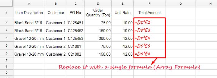
How do we convert those non-array formulas into an array formula in cell F2 that spills down?
Array Formula in Google Sheets Using the Function ARRAYFORMULA:
Double-click on cell F2 and insert the following formula.
=ArrayFormula(D2:D6*E2:E6)Or
Double-click on cell F2 and type =D2:D6*E2:E6 and then hit the Google Sheets keyboard shortcut Ctrl+Shift+Enter. By doing so, Google Sheets will automatically insert the ARRAYFORMULA function.
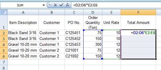
Excel Array Formula Using Curly Braces:
The Excel array formula approach (legacy array formula) is entirely different, and I find Google Sheets to be more user-friendly than Excel in this case.
Excel typically requires the keyboard shortcut approach, although Excel in Office 365 and Excel 2019 is an exception.
In Excel, select the cell range F2:F6.
Type the formula =D2:D6*E2:E6 and then hit Ctrl+Shift+Enter.
I have detailed above the difference in the application of array formulas in Excel and Google Sheets. Now, here is the aftereffect.
Editing Array Formula Ranges:
Excel:
When attempting to delete or insert rows within this formula range, you will receive the following notification:
“You Cannot Change Part Of An Array.”
Then, how can I edit the Excel legacy array formula range?
- Select the cells containing the formula (in this example, it’s F2:F6).
- Hit delete.
If you prefer, you can copy the formula before deleting it. Now you can make changes to individual cells.
Google Sheets:
In Google Sheets, you can insert or delete rows within the formula range.
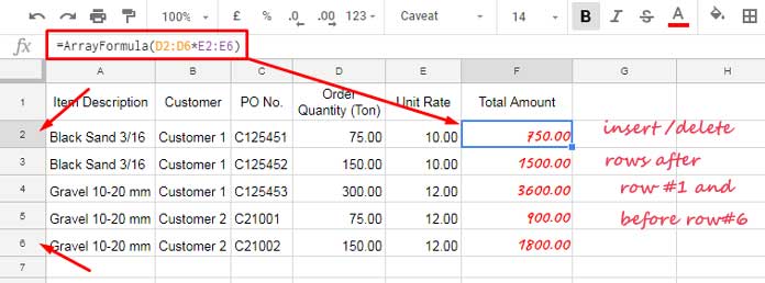
The formula will automatically cover the newly inserted rows with no warning messages or restrictions.
In this regard, the Google Sheets array formula excels.
Infinite Ranges in Array Formula in Google Sheets and Excel
Google Sheets array formulas support infinite/open-ended ranges like A1:A or A10:Z.
Example:
=ArrayFormula(D2:D*E2:E)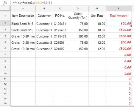
The above formula in cell F2 may populate unwanted values in blank rows. To address this issue, when using infinite ranges, it is advised to use an IF + LEN combo together with the array formula as below:
=ArrayFormula(IF(LEN(A2:A), D2:D*E2:E, ))In Excel, both ends of the range should be open, as in A:A.
Single-Cell or Non-Expanding Array Formulas
Some array formulas, specifically combination formulas, don’t expand their result.
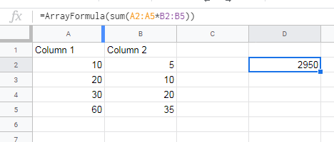
For example, when you multiply two arrays and sum, the formula will return a single aggregated value. Here is an example of such a non-expanding/single-cell array formula in Google Sheets:
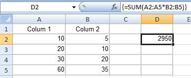
=ArrayFormula(SUM(A2:A5*B2:B5))In Google Sheets, you just need to enter the formula in any cell, for example, cell D2.
In Excel, you need to enter the formula in cell D2 and press Ctrl+Shift+Enter.
That’s all about the usage of array formulas in Google Sheets and Excel.
ArrayFormula Function Alternatives in Google Sheets
In Google Sheets, the function ARRAYFORMULA is not a must to handle expanding array results! Yes! You heard me right.
Let me explain with an example.
The following formula will return the column numbers 1 to 10 horizontally.
=ArrayFormula(COLUMN(A1:J1))Here you can replace the ARRAYFORMULA with the INDEX function as below.
=INDEX(COLUMN(A1:J1))Conclusion
As I mentioned at the beginning, we can’t convert all non-expanding formulas to expanding ones. For example, to expand functions like SUM, COUNT, AVERAGE, etc., you may need to utilize LAMBDA helper functions (LHF) or other row-wise array workarounds that involve database functions.
These functions (LHF) can even expand the results of functions capable of returning 2D arrays, such as FILTER in both Excel and Google Sheets.
You can find a great example in my following Google Sheets Tutorial: Conquer Duplicate IDs: Master Left, Right, Inner, & Full Joins in Google Sheets.
That’s all about how array formulas differ in Google Sheets and Excel. I hope you enjoyed the journey.


Thanks, Prashant for your efforts! Just needed it to understand what happened, importing an excel file to Sheets 🙂
Can Excel array formulas output multi-cell results? If not, that is the single most significant difference not stated in the article.
Isn’t the
=ArrayFormula(sum(A2:A4)*sum(B2:B4))the same as just=sum(A2:A4)*sum(B2:B4)?Sorry for the error!
I meant to say
=ArrayFormula(sum(A2:A4*B2:B4))Thanks for notifying me.
I have updated the post to incorporate the change.