A handy Vlookup tutorial to let you know how you can make Vlookup skips hidden rows in Google Sheets.
To Vlookup only visible rows in Google Sheets, you must use a helper column that contains a Subtotal formula.
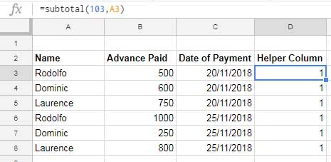
Assume you have a sample data in A2: C8 and if so you can use the column range D2: D8 as the helper column.
In that case, in Cell D3 use the below Subtotal formula and copy (drag) that formula up to the cell D8.
=subtotal(103,A3)
This formula would return the value 1 in rows that are visible and 0 in hidden rows.

Hope you have completed the above steps. Now let us Vlookup visible rows in Google Sheets.
Formula Example: Vlookup Skips Hidden Rows in Google Sheets
Search Key: Dominic (the search key must be from the first column)
Index Column: 2 (Column B) (the formula returns a value from this column.
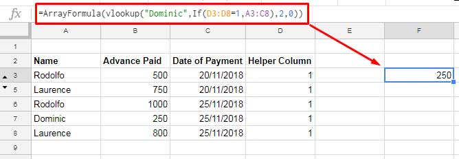
The name “Dominic” is in cell A4 and A7. I am hiding the row#4. The following regular Vlookup formula would return the value 600, which is in cell B4 hidden.
=vlookup("Dominic",A3:C8,2,0)
Then what is the correct Vlookup formula to skip hidden rows in Google Sheets?
Formula:
=ArrayFormula(vlookup("Dominic",If(D3:D8=1,A3:C8),2,0))
Screenshot:

How this Vlookup formula excludes hidden rows in lookup?
The helper column plays a vital role in the above Vlookup. As you can see, instead of using A3: C8 as the Vlookup range, I have used a Logical IF statement that makes use of the values in helper column. Here is that formula.
If(D3:D8=1,A3:C8)
If you key in this formula in any cell, it won’t work correctly. It requires ArrayFormula to populate the below data.
Note: In a combination formula, if there is an ArrayFormula requirement inside it you can move it to the first part of the formula. This opens a new possibility. If there are multiple ArrayFormulas, in most of the cases you can remove all of them and use a single ArrayFormula in the first part.
Array Formula:
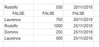
=ArrayFormula(If(D3:D8=1,A3:C8))
Output:

As you can observe the values in the hidden rows are FALSE. So the Vlookup search key won’t match in this row.
This way you can make the Vlookup Skips Hidden Rows in Google Sheets.
More Resources:
1. Google Sheets Query Hidden Row Handling with Virtual Helper Column.
2. SUMIF Excluding Hidden Rows in Google Sheets [Without Helper Column].
3. How to Omit Hidden or Filtered Out Values in Sum [Google Doc Spreadsheet].
4. Count Unique Values in Visible Rows in Google Sheets.
5. Find the Average of Visible Rows in Google Sheets.
6. Subtotal Function With Conditions in Excel and Google Sheets.


