We should use the COUNTUNIQUEIFS function, not COUNTUNIQUE, to count unique values in visible rows only in Google Sheets.
When we filter data to focus on specific records, most functions include hidden rows in their calculations. However, there is a technique to exclude hidden rows.
You should replace your ‘intended’ function with an alternative function that supports criteria usage.
Because we need to include a virtual helper column that contains 1 (visible) and 0 (hidden) to identify hidden rows, we should be able to specify helper_column>=1 as a criterion.
That’s why we use COUNTUNIQUEIFS instead of COUNTUNIQUE.
First, let’s see how COUNTUNIQUE behaves with filtered data.
My sample data in D1:D10 consists of 6 unique values, excluding the header, before filtering.
=COUNTUNIQUE(D2:D10)
Now, let’s apply a filter to this range and see what happens.

The formula still returns 6, even though I have filtered out a few rows. Below, you can see the solution to count unique values in visible rows in Google Sheets.
Counting Unique Values in Visible Rows
We will start with data in a single column, and then proceed to more than one column.
Syntax of the COUNTUNIQUEIFS Function in Google Sheets:
COUNTUNIQUEIFS(range, criteria_range1, criterion1, [criteria_range2, …], [criterion2, …])Assume D2:D is the range where you want to count unique values in visible rows. You can use the following formula, where D2:D is provided as an example that you should replace with your actual range.
=COUNTUNIQUEIFS(D2:D, MAP(D2:D, LAMBDA(r, SUBTOTAL(103, r))), 1)Where:
range: D2:Dcriteria_range:MAP(D2:D, LAMBDA(r, SUBTOTAL(103, r))), which returns 1 for visible rows and 0 for hidden rowscriterion: 1
Note: You can repeat the criteria_range and criterion for additional filtering conditions.
Explanation of the criteria_range
We can use SUBTOTAL(103, D2) to check if the value in cell D2 is counted. The function number 103 in SUBTOTAL represents COUNTA. When you hide row #2, D2 becomes invisible. Thus, the output of the SUBTOTAL formula will be 0.
We can use the LAMBDA function to create a custom function that checks visibility: LAMBDA(r, SUBTOTAL(103, r)). Here, ‘r’ represents the current element being processed by the function.
LAMBDA(r, SUBTOTAL(103, r))To apply this to the range D2:D, we use the MAP lambda helper function.
Syntax:
MAP(array1, [array2, …], lambda)By specifying the array D2:D, MAP will map each value within the custom function and return an array output.
Counting Unique Values in Visible Rows in Multiple Columns
Sometimes you may want to count unique values based on two or more columns.
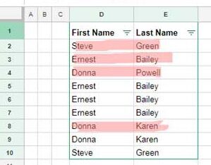
For example, you might want to get the count of unique employees in visible rows when the employees’ first and last names are in two columns.
Here, the COUNTUNIQUEIFS function won’t work because combining first and last names as a criteria range will cause an “Argument must be a range” error.
Instead, we will extract visible rows using the FILTER function and apply UNIQUE to it. This will return the unique records. Then, we count the values in one of the columns using COUNTA.
In the following example, the first names are in column D and the last names are in column E. Here is the formula to count unique names in visible rows:
=COUNTA(
   CHOOSECOLS(
      UNIQUE(
         FILTER(D2:E, MAP(D2:D, LAMBDA(r, SUBTOTAL(103, r)))=1)
       ), 1
   )
)
Formula Explanation
FILTER(D2:E, MAP(D2:D, LAMBDA(r, SUBTOTAL(103, r)))=1): Filters the range D2:E where the virtual helper column returns 1 (indicating visible rows).UNIQUE(…): Returns the unique rows from the above filter formula result.CHOOSECOLS(…, 1): Returns the first column from the unique rows.COUNTA(…): Returns the count of the unique values.
In this formula, you can replace D2:E with your actual table range.
That’s all about counting unique rows in a multiple-column range in Google Sheets.
Resources
Here are some Google Sheets tutorials that help handle hidden rows in calculations:
- Find the Average of Visible Rows in Google Sheets
- IMPORTRANGE to Import Visible Rows in Google Sheets
- XLOOKUP Visible (Filtered) Data in Google Sheets
- XMATCH Visible Rows in Google Sheets
- Weighted Average of Filtered (Visible) Data in Google Sheets
- UNIQUE Function in Visible Rows in Google Sheets
- How to Omit Hidden or Filtered Out Values in SUM
- SUMIF Excluding Hidden Rows in Google Sheets
- Google Sheets Query Hidden Row Handling with Virtual Helper Column
- Vlookup Skips Hidden Rows in Google Sheets – Formula Example
- Insert Sequential Numbers Skipping Hidden | Filtered Rows in Google Sheets
- COUNTIF | COUNTIFS Excluding Hidden Rows in Google Sheets
- How to Exclude Manually Hidden Rows from a Pivot Table in Google Sheets


This is perfect for what I needed, but can you explain to me the formula for counting VISIBLE cells in a column that have a specific text? The current formula I am using is
=COUNTIF(O8:O, "Text"), but this does not adjust when I filter out data. I appreciate any help I can get! Thank you!Please see the resource section at the end of this tutorial for the relevant COUNTIF | COUNTIFS tutorial.