COUNTUNIQUEIFS in Google Sheets: Syntax, Examples & Multiple Criteria

Using the COUNTUNIQUEIFS function, we can conditionally count unique values in a data range in Google Sheets.

Before the introduction of COUNTUNIQUEIFS, we used a combination of COUNTUNIQUE and FILTER to conditionally count unique values. The FILTER function filtered the range based on the specified conditions, and COUNTUNIQUE returned the number of distinct values in the filtered result. That workaround is no longer necessary.

Table of Contents

At a Glance

Here are the most common COUNTUNIQUEIFS formulas.

Task	Formula
Count unique values with one condition	`=COUNTUNIQUEIFS(B2:B, A2:A, E2)`
Count unique values with multiple AND conditions (criteria in different columns)	`=COUNTUNIQUEIFS(A2:A, B2:B, ">100", C2:C, "Delivered")`
Count unique values with multiple AND conditions in the same column (comparison criteria)	`=COUNTUNIQUEIFS(B2:B, C2:C, ">=10", C2:C, "<=20")`
Count unique values with OR conditions (criteria list)	`=ARRAYFORMULA(COUNTUNIQUEIFS(B2:B, XMATCH(A2:A, D2:D3), ">0"))`

The following sections explain each formula with practical examples.

COUNTUNIQUEIFS Syntax and Arguments

Here are the syntax and arguments of the COUNTUNIQUEIFS function in Google Sheets.

Syntax:

COUNTUNIQUEIFS(range, criteria_range1, criterion1, [criteria_range2, …], [criterion2, …])

Arguments:

range: The range or array from which to count unique values.
criteria_range1: The range or array in which to evaluate criterion1.
criterion1: The condition to apply to criteria_range1.
Additional criteria_range and criterion pairs are optional and follow the same pattern.

If the arguments seem confusing, don’t worry. The following examples explain how each argument works.

COUNTUNIQUEIFS: Basic Example

Assume three individuals participated in an athletics event, specifically the long jump, and their performances (distance jumped) have been recorded in Google Sheets. Each person has three scores because they jumped three times.

Out of curiosity, I want to find the count of unique (distinct) performances for each individual. Let’s see how to achieve this using the COUNTUNIQUEIFS function.

The athletes’ names (criteria_range1) are in cells A2:A, and their distances jumped (range) are in cells B2:B. Enter any athlete’s name (criterion1) in cell E2, and then use the following formula in cell F2:

=COUNTUNIQUEIFS(B2:B, A2:A, E2)

Basic Example of the COUNTUNIQUEIFS Function in Google Sheets

The formula returns 2 when the criterion in cell E2 is “John.”

John’s recorded distances are 8.2 m, 8 m, and 8.2 m. Since there are only two distinct values, the formula returns 2.

This is a basic example of using the COUNTUNIQUEIFS function to conditionally count unique values in Google Sheets.

COUNTUNIQUEIFS with Multiple Conditions

In the previous example, we applied a condition to a single column, specifically the range containing the athletes’ names.

However, you may sometimes need to apply multiple conditions in the same column or across two or more different columns.

Let’s see how to handle multiple conditions using COUNTUNIQUEIFS.

Multiple AND Conditions in Different Columns

Consider a dataset containing fruit names in column A, order quantities in column B, and delivery status in column C.

I want to find the unique count of fruits with quantities greater than 100 and the status “Delivered.” This means we need to apply two conditions while counting unique values.

Formula:

=COUNTUNIQUEIFS(A2:A, B2:B, ">100", C2:C, "Delivered")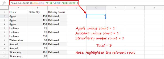

Using COUNTUNIQUEIFS with Multiple AND Conditions in Google Sheets

That’s all it takes to apply multiple conditions in different columns using COUNTUNIQUEIFS.

Multiple AND Conditions in the Same Column

Suppose I have three employees—Anwesha, Swetha, and Kiran—and I have assigned multiple tasks to them.

Task ID	Developer	Estimated Hours
T1	Anwesha	8
T2	Kiran	6
T3	Swetha	11
T4	Swetha	10
T5	Kiran	11
T6	Anwesha	7

I want to find the number of unique employees who have been assigned tasks with estimated hours between 10 and 20.

Use the following formula:

=COUNTUNIQUEIFS(B2:B, C2:C, ">=10", C2:C, "<=20")

The formula returns the unique count of employees whose estimated hours fall between 10 and 20.

OR Conditions (Criteria List)

In the previous example, we used comparison operators in the criteria. However, there are situations where COUNTUNIQUEIFS alone cannot handle the required condition.

Consider the following purchase dataset.

Date	Item	Qty
5/7/2026	Apple	5
5/7/2026	Apple	5
6/7/2026	Apple	4
12/7/2026	Apple	10
12/7/2026	Mango	5
12/7/2026	Mango	6

I want to find the number of unique items received on 5/7/2026 or 12/7/2026 in a single formula.

The sample data is in A1:C, and the criteria dates (5/7/2026 and 12/7/2026) are in D2:D3.

Use the following formula:

=ARRAYFORMULA(COUNTUNIQUEIFS(B2:B, XMATCH(A2:A, D2:D3), ">0"))

The XMATCH function matches each date against the criteria list. It returns the relative position of each matching date and #N/A for non-matching rows.

The result returned by XMATCH becomes the criteria_range, while the criterion ">0" selects all matching rows.

ARRAYFORMULA is required because XMATCH evaluates multiple lookup values.

FAQ

Can COUNTUNIQUEIFS use OR conditions?

Not directly. You can use XMATCH, MATCH, or REGEXMATCH to identify the matching rows first, and then use the result as the criteria range in COUNTUNIQUEIFS.

Can COUNTUNIQUEIFS count unique values in multiple columns?

No. COUNTUNIQUEIFS can count unique values from only one range. If you specify multiple ranges as the first argument, it returns a #VALUE! error stating: “Array arguments to COUNTUNIQUEIFS are of different sizes.”

What’s the difference between COUNTUNIQUEIFS and COUNTUNIQUE?

Use COUNTUNIQUE to count unique values in a range. Use COUNTUNIQUEIFS when you want to count unique values that meet one or more conditions.

10 COMMENTS

Dhananjai Kumar April 14, 2022 At 8:10 am

How to use multiple criteria from the same column in the COUNTUNIQUEIFS formula?

I want to count 2 different values from 1 column and put time criteria from the other column.

- Prashanth April 14, 2022 At 7:03 pm
  
  Hi, Dhananjai Kumar,
  
  You may please try to share a sample sheet below in your reply.
  
Aditya Darekar July 18, 2020 At 12:29 am

Hi Prashanth

I wanted to know why Countuniqueifs formula doesn’t expand when used with ArrayFormula like other functions such as IFS or SUMIF etc.

I have three columns. Col A is for dates, Col B is for operators and Col C is the product they have handled. There are almost 15 to 20 entries with the same date and the operator handled 3 to 4 different products.

I wanted to know the number of operators worked on a particular date. I have used a Unique formula to get the dates and using Countuniqueifs formula to get the number of operators present for that day.

It works when used in a single cell but doesn’t expand when used with an array formula.

Any suggestion?

- Prashanth July 18, 2020 At 10:25 am
  
  Hi, Aditya Darekar,
  
  Similar to SUMIFS it seems the COUNTUNIQUEIFS won’t work with the ArrayFormula to expand. You can try this Unique and Query combination.
  
  =query(unique(A1:B),"Select Col1,count(Col2) where Col1 is not null group by Col1")
  
  - Aditya Darekar July 18, 2020 At 3:57 pm
    
    Thanks, Prashanth,
    
    I have tried but it is not giving me the unique values count rather it is giving me total count.
    
    - Prashanth July 18, 2020 At 5:18 pm
      
      Can you share your sheet, please? The link will be safe (I won’t publish it). Only share a mockup sheet.
      
      - Aditya Darekar July 18, 2020 At 5:47 pm
        
        Thanks a lot, Prashanth… It is working.
        
        Actually, later on, I have added one more column for Item name in Col B so my column B shifted to Col C. So I just altered in the formula to C and Col3.
        
        =query(unique(A1:C),"Select Col1,count(Col3) where Col1 is not null group by Col1")
        
        But didn’t work.
        
        Now just changed to
        
        =query(unique({A1:A,C1:C}),"Select Col1,count(Col2) where Col1 is not null group by Col1")
        
        IT WORKED!!!!
        
        
        Prashanth July 19, 2020 At 8:35 am
        
        Hi, Aditya Darekar,
        
        That’s because of the Unique().
        
        Thanks for your feedback!
        
Pablo September 15, 2019 At 5:50 am

Hello Prashanth,

Thank you for your tutorials they have been very helpful. You have given an example for date criterion within the formula, however, what if the dates are part of the table?

Let’s say in your fruit table example your columns B and C were actually two dates. In a separate cell, I’d like to enter a date for which unique fruits in column A are counted if the date entered is between the 2 dates given in columns B and C. Is this still possible using the COUNTUNIQUEIFS function?

Thanks!

- Prashanth September 15, 2019 At 9:31 am
  
  Hi Pablo,
  
  Assume the date criterion for COUNTUNIQUEIFS is in cell E2. Then the formula would be as follows.
  
  Date range in Countuniqueifs function:
  
  Best,