Are you trying to use COUNTUNIQUEIFS as an array formula in Google Sheets?
If yes, you might have noticed that the dedicated COUNTUNIQUEIFS function does not return row-wise expanding results. But don’t worry—there are workarounds.
In this tutorial, I’ll show you three effective methods to achieve row-wise COUNTUNIQUEIFS in Google Sheets:
- A drag-down approach with helper columns.
- An array formula solution using MAP + LAMBDA.
- An alternative using QUERY and SORTN.
Example Scenario – Workshop Attendance
Imagine you’re tracking which sessions participants attended in a 3-day workshop:
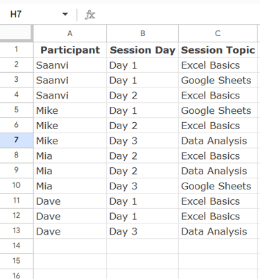
Goal: Count how many unique session topics each participant attended.
Expected results:
- Saanvi → 2 (Excel Basics, Google Sheets)
- Mike → 3 (Google Sheets, Excel Basics, Data Analysis)
- Mia → 3 (Excel Basics, Data Analysis, Google Sheets)
- Dave → 2 (Excel Basics, Data Analysis)
Option 1 – Row-Wise COUNTUNIQUEIFS (Non-Array Drag-Down Formula)
This approach uses helper columns and drag-down formulas.
In E2, enter:
=TOCOL(UNIQUE(A2:A), 1)This extracts the unique list of participants while removing any blank rows.
In F2, enter:
=COUNTUNIQUEIFS($C$2:$C, $A$2:$A, E2)Drag down, and you’ll get the unique session count for each participant.

✅ Works fine, but this method is not a pure array formula.
Option 2 – Row-Wise COUNTUNIQUEIFS Using MAP + LAMBDA
With the new MAP and LAMBDA functions, we can create a fully self-expanding array formula.
Keep the earlier E2 formula as it is. Then, in F2, enter:
=MAP(
  TOCOL(UNIQUE(A2:A), 1),
  LAMBDA(uPart, COUNTUNIQUEIFS(C2:C, A2:A, uPart))
)
Explanation:
TOCOL(UNIQUE(A2:A), 1)→ extracts unique participants.MAPiterates through each participant.LAMBDAappliesCOUNTUNIQUEIFSfor each participant.
✅ No need to drag formulas manually. This is the cleanest array-based approach.
Option 3 – Row-Wise COUNTUNIQUEIFS Using QUERY + SORTN
If you want an alternative without explicitly setting criteria, QUERY + SORTN works beautifully.
In E2, enter:
=QUERY(
   SORTN(A2:C, 9^9, 2, 1, TRUE, 3, TRUE),
   "SELECT Col1, COUNT(Col3) WHERE Col1 <>'' GROUP BY Col1 LABEL COUNT(Col3)''"
)
How it works:
SORTN(A2:C, 9^9, 2, 1, TRUE, 3, TRUE)→ creates unique combinations of Participant (Col1) and Session Topic (Col3).9^9→ arbitrarily large number, ensuring all rows are considered.2→ tie-breaking mode that removes duplicates based on the sort columns.1, TRUE, 3, TRUE→ sort by column 1 (Participant) and column 3 (Topic).
QUERY→ groups the results by Participant (Col1) and counts unique topics (Col3).
✅ This approach automatically counts unique topics per participant without helper columns.
Bonus: Listing Unique Topics Instead of Just Counting
So far, we’ve learned how to count the number of unique session topics each participant attended.
But what if you want to actually list out those unique session topics per participant instead of just counting them?
You can achieve this with the same QUERY + SORTN combo, using a slightly different query string:
=QUERY(
  SORTN(A2:C, 9^9, 2, 1, TRUE, 3, TRUE),
  "SELECT MAX(Col3) WHERE Col3 <> '' GROUP BY Col3 PIVOT Col1"
)
How it works:
SORTNensures each unique combination of Participant (Col1) and Session Topic (Col3) is included once.- The
QUERYthen pivots the data:GROUP BY Col3→ groups results by topic.PIVOT Col1→ creates participant-wise columns, showing which participant attended each unique topic.
MAX(Col3)is just a trick here—it returns the topic name itself in each row.
Result:
| Dave | Mia | Mike | Saanvi |
| Data Analysis | Data Analysis | Data Analysis | |
| Excel Basics | Excel Basics | Excel Basics | Excel Basics |
| Google Sheets | Google Sheets | Google Sheets |
Frequently Asked Questions (FAQs)
What does COUNTUNIQUEIFS do in Google Sheets?
It counts the number of unique values in a range, filtered by one or more conditions.
Can I use COUNTUNIQUEIFS as an array formula?
Not directly. COUNTUNIQUEIFS by itself doesn’t spill results across rows. Instead, you can combine it with MAP + LAMBDA or use QUERY + UNIQUE/SORTN for row-wise array solutions.
What’s the difference between COUNTUNIQUE and COUNTUNIQUEIFS?
COUNTUNIQUE counts unique values in a range with no conditions.
COUNTUNIQUEIFS allows conditions (e.g., unique items per participant or date).
Which approach is best for row-wise COUNTUNIQUEIFS?
Personally, I recommend the MAP + LAMBDA approach as the most modern and elegant solution. The QUERY method is an excellent fallback.
Wrap-Up
The COUNTUNIQUEIFS function alone doesn’t work in an array-expanding manner, but you can still achieve row-wise results in Google Sheets using:
- Drag-down helper method (basic but manual).
- MAP + LAMBDA (modern, elegant).
- QUERY + SORTN (practical and flexible).
I recommend the MAP + LAMBDA approach for a clean, self-expanding formula.
And if you’d like to go beyond counting, you can also use QUERY + SORTN to list the actual unique topics per participant, not just the counts.


While all these methods work, I feel the best way to do this task is using a pivot table.
Hi, S K Srivastava,
I agree with you. We can use the COUNTUNIQUE within the Pivot Table. But I prefer to experiment with formulas 🙂