SORTN is one of the powerful functions in Google Sheets that every Sheets enthusiast should learn. It’s not just for sorting.
The purpose of the SORTN function is to return the first n records in a data set after sorting by one or more columns.
Even if we specify ‘n’, the output may not exactly match ‘n’ if there are fewer records to return or multiple occurrences of values in the sort by column.
The function sorts the data by values in the sort by column. When there are duplicates in this column, you can control whether to return all duplicates or just the first occurrence using the display ties mode.
The examples below, along with screenshots, will give you a clear understanding of how to use the SORTN function in Google Sheets.
A Well-Curated Sample Data for Testing the SORTN Function
Understanding the SORTN function can be quite tricky. It requires a balanced sample dataset to help you understand all its arguments. The following sample data is sufficient to explain this powerful function in Google Sheets.
Sample Data (Range A1:C):
| Student Name | Marks | Grace Marks |
| Christine | 85 | 5 |
| Linda | 85 | 0 |
| Steven | 90 | 0 |
| Annie | 90 | 4 |
| Christopher | 90 | 5 |
| Randy | 95 | 0 |
| Albert | 95 | 0 |
| Nicholas | 95 | 0 |
| Keith | 99 | 0 |
Note: This sample data is for demonstration purposes, and real-world data structures might vary.
Syntax of the SORTN Function
SORTN(range, [n], [display_ties_mode], [sort_column1, is_ascending1], …)All arguments except the range are optional. Let’s learn about them in detail below.
Mastering Selective Data Retrieval with SORTN
range: The range to sort
‘range’ is the data range to sort, and you should exclude the header row when specifying it.
=SORTN(A2:C)This formula will return the following record because the default output will contain 1 row, sorted by column 1 in ascending order.
| Albert | 95 | 0 |
n: The Number of Rows to Return
The second argument in the SORTN function is for specifying the number of rows you want in the result.
=SORTN(A2:C, 2)This will return the following two records sorted by column 1 in ascending order:
| Albert | 95 | 0 |
| Annie | 90 | 4 |
When you are unsure about the number of rows in your ‘range’ to sort and want all the rows in the result, specify 9^9, an arbitrarily large number. Because ‘n’ can be any number greater than 0.
display_ties_mode, sort_column, and is_ascending: Control Ties in the SORTN Function
These three arguments are inseparable. You should specify all of them to control ties (multiple occurrences of values in the sort by column).
The four display_ties_mode options in the SORTN function are 0, 1, 2, and 3.
The display_ties_mode controls the output when ties (multiple occurrences of values) occur in the sort_column.
The sort_column is the first column in the range by default. However, when you specify display_ties_mode, you should also specify the sort_column.
The default sort order (is_ascending) is TRUE (ascending), but you should specify it as well when using the display_ties_mode.
display_ties_mode 0
The default display_ties_mode is 0, which is neutral. It means it returns ‘n’ rows without removing duplicate records. In all the above examples, we haven’t specified the ties mode, so it considers the default value, which is 0.
The following formula will return 3 students with the lowest marks:
=SORTN(A2:C, 3, 0, 2, TRUE)The below one will return three students with the highest marks:
=SORTN(A2:C, 3, 0, 2, FALSE)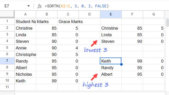
These records do not reflect the top three or bottom three scorers as there are other students with the same marks. These formulas simply return the first 3 rows in the sorted range.
Note:
In the SORTN function, you can specify the sort_column by column index or column reference. For example, you can use =SORTN(A2:C, 3, 0, 2, TRUE) or =SORTN(A2:C, 3, 0, B2:B, TRUE). Similarly, you can specify TRUE or 1 for ascending sort and FALSE or 0 for descending sort.
display_ties_mode 1
This mode extracts the first ‘n’ rows and includes any additional rows that have identical values to the nth row in the result set. It is less commonly used.
The following formula will return 2 students with the lowest marks plus any student who has the same mark as the second lowest mark:
=SORTN(A2:C, 2, 1, 2, TRUE)The following formula will return 2 students with the highest marks plus any student who has the same mark as the second highest mark:
=SORTN(A2:C, 2, 1, 2, FALSE)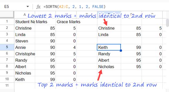
display_ties_mode 2
This mode is most popular as it helps remove duplicates by analyzing specific columns in Google Sheets.
Use this mode to return at most the first ‘n’ rows after removing duplicate rows.
This formula returns the lowest 3 marks, excluding duplicates:
=SORTN(A2:C, 3, 2, 2, TRUE)This formula returns the highest three marks, excluding duplicates:
=SORTN(A2:C, 3, 2, 2, FALSE)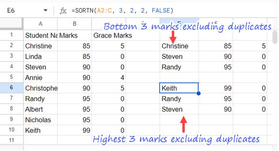
display_ties_mode 3
Use this mode in the SORTN function to extract the first ‘n’ records and include all duplicates. It is useful when you want to retain all occurrences of values.
This formula returns the lowest 2 marks, including duplicates:
=SORTN(A2:C, 2, 3, 2, TRUE)This formula returns the top 2 marks, including duplicates:
=SORTN(A2:C, 2, 3, 2, FALSE)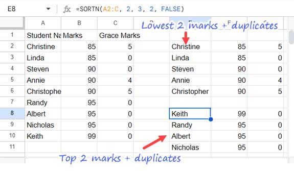
Breaking Ties Using Additional Sort By Column in the SORTN Function
In our sample data, I’ve purposefully added a Grace Marks column. Let’s see how to break a tie using this when students have the same marks in the Marks column.
The following SORTN formula will return the top 3 marks excluding duplicates:
=SORTN(A2:C, 3, 2, 2, FALSE)It will return the following records:
| Keith | 99 | 0 |
| Randy | 95 | 0 |
| Steven | 90 | 0 |
As you can see in the sample data, two more students have a score of 90. Since they are duplicates and not the first occurrence, SORTN removed them:
| Steven | 90 | 0 |
| Annie | 90 | 4 |
| Christopher | 90 | 5 |
To break the tie using the Grace Marks column, which is the third column, you can use:
=SORTN(A2:C, 3, 2, 2, FALSE, 3, FALSE)| Keith | 99 | 0 |
| Randy | 95 | 0 |
| Christopher | 90 | 5 |
This formula will consider the grace marks of students when there is a tie in their marks.
SORT and SORTN Functions Combo Use in Google Sheets
Using SORTN with SORT is very common. We first sort the data in the preferred order and then apply the SORTN function.
This is most useful when you want to extract the last records from a table.
In the following example, I have the Tested Time, Tested Date, and Tested By columns. The range is A1:C.
I want to return the latest records so that I can understand the last tested time each day and the person.
| Tested Time | Tested Date | Tested By |
| 2024-06-20 10:10 | 20/06/2024 | Olivia |
| 2024-06-20 12:10 | 20/06/2024 | Jack |
| 2024-06-20 14:10 | 20/06/2024 | Rose |
| 2024-06-21 10:05 | 21/06/2024 | Olivia |
| 2024-06-21 11:40 | 21/06/2024 | Rose |
| 2024-06-21 15:00 | 21/06/2024 | Jack |
Here we should first sort the data by column 1 in descending order and use that within the SORTN function as the range argument. Here is the formula:
=SORTN(SORT(A2:C, 1, FALSE), 9^9, 2, 2, TRUE)Note: Specifying 9^9 (a large number) for n is a workaround for cases where you’re unsure about the number of rows and want all results.
Result:
| 2024-06-20 14:10 | 20/06/2024 | Rose |
| 2024-06-21 15:00 | 21/06/2024 | Jack |
That’s all about using the SORTN function in Google Sheets.


