Can I filter unique values/rows/records using the Filter Menu in Google Sheets? Is it possible?

Yes! you can filter unique values using the Filter menu in Google Sheets. Utilize a custom formula in the Filter menu’s custom formula field, similar to how you use custom formulas in conditional formatting.

When you filter your data using the Filter menu command interface, it offers several advantages. One of the foremost benefits is filtering your data at the source, allowing direct editing of the filtered data.

Besides the Filter menu, Google Sheets provides functions like FILTER and QUERY for conditional data filtering. However, these functions don’t enable filtering data at its source; they filter data into a new range or sheet.

It’s important to note that these functions lack parameters for making the data unique. You may consider using UNIQUE or SORTN in conjunction with these functions to achieve uniqueness.

In this discussion, our focus is on filtering unique values using the Filter menu. This can be accomplished by utilizing a custom formula in the Filter menu’s custom formula field, which applies to both sorted and unsorted data.

Sample Data (Sorted)

First, I’ll apply my custom formula to a sorted list so you can grasp the concept.

The sample data includes authors’ names in column A and their book titles in column B. As the data is sorted, you can readily identify repeated book titles in column B.

Now, let’s explore how to filter unique values—specifically, book titles—using the Filter menu.

How to Filter Unique Values Using the Filter Menu

Before filtering unique values using the Filter menu, decide whether you want to filter the first occurrence or the last.

For instance, let’s consider the book title “The Mysterious Affair at Styles,” which appears in rows 5, 6, and 7. Which row would you like to see, the 5th or the 7th?

If you want to filter the first occurrence, use this formula:

=COUNTIF($B$1:B2, B2)=1

If you want to filter the last occurrence, use this formula:

=COUNTIF(B2:B, B2)=1

Both COUNTIF formulas can effectively filter unique values in the Filter menu. The output will be the same, but there’s a difference when you examine the rows.

Both formulas follow the syntax:

COUNTIF(range, criterion)

In the first formula, the range includes the header row and the row below it ($B$1:B2), while in the second formula, the range encompasses the entire column except for the header (B2:B).

Note: To understand what these formulas return, enter them in cell C2 and drag the fill handle down as far as needed.

Step-by-Step Instructions

1. Select the data range, here, A1:B16 or A1:B.
2. Go to the Data menu and click on “Create a filter.”
   
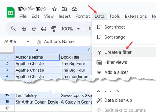
3. Navigate to cell B1 and click on the filter drop-down, then select “Filter by condition” > “Custom formula is.”
   
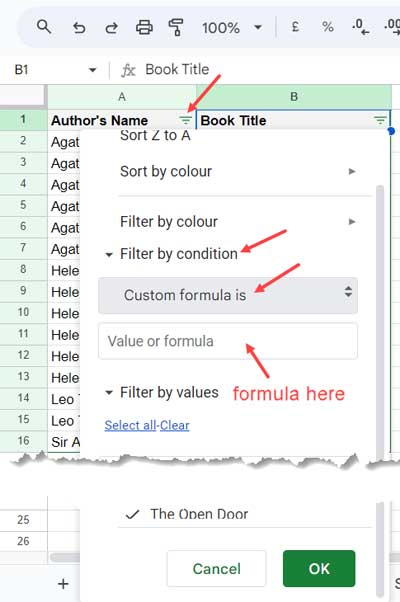
4. In the given field, enter one of the above COUNTIF formulas and click OK.

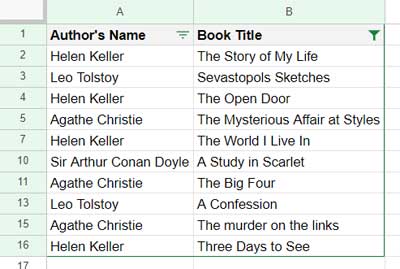
This will filter the unique rows in column B.

Filtering Unique Values in Unsorted Data Using Filter Menu

Do I need to sort the data before applying the above custom formulas in the Filter menu?

No, you don’t! You can use the same formulas. So needless to say, all the steps are the same.

The formulas will correctly filter the unique records.

Resources

Here are some related resources regarding the filter menu in Google Sheets.

1. How to Filter by Month Using the Filter Menu in Google Sheets
2. Filter by Date Range Using Filter Menu in Google Sheets
3. Filter Menu to Filter Max N Values in Google Sheets – Custom Formula
4. Using Cell Reference in Filter Menu Filter by Condition in Google Sheets