Want to use a cell reference inside the filter menu in Google Sheets — specifically in the “Filter by condition” > “Custom formula is” section? It’s not super obvious how it works, but once you know the trick, it’s quite handy.
I’ll walk you through two simple examples to show the proper way to use cell references in the Filter menu.
A Quick Intro to the Filter Menu in Google Sheets
Google Sheets has two powerful functions — FILTER and QUERY — to help you slice and dice data. But not everyone wants to write a formula just to filter something.
That’s where the Filter menu (under Data) comes in. You can use it to quickly filter a dataset without creating a new table or adding formulas.
There are two filter options:
- Create a filter – for quick one-time filters.
- Create a filter view – for saved, reusable views (also lets multiple people apply their own filters without affecting others).
Now, let’s see how to use a cell reference inside the filter menu — specifically under Custom formula is.
Using Cell References in Filter Menu: Two Ways
You can use a formula inside the filter menu to:
- Check a condition directly (e.g., if the value equals “Jesse”)
- Refer to a cell that holds the condition (e.g., $E$1 contains “Jesse”)
Let’s see both with an example.
Example Dataset
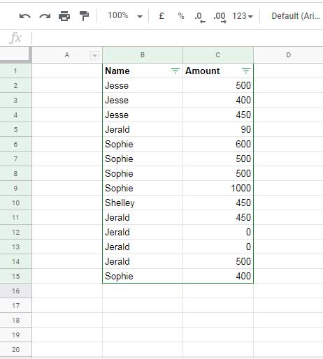
Say you have data in B1:C15 with names in column B and amounts in column C (like advance, salary, etc.).
- Select B1:C15
- Go to Data > Create a filter
Now you can use the dropdown in B1 to set up a filter condition.
Example 1: Hardcoded Condition in Custom Formula
You want to filter names that are exactly “Jesse”.
- Click the filter dropdown in cell B1
- Choose Filter by condition > Custom formula is
- Enter:
=B2="Jesse"
(Don’t use=B2:B15="Jesse"orARRAYFORMULAhere — just start from the top cell in the column, B2.) - Click OK to apply the filter
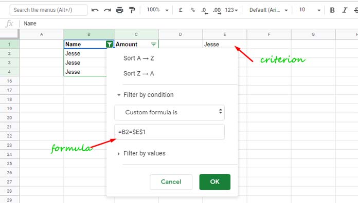
Example 2: Refer to a Cell for the Filter Value
Let’s say you enter the name “Jesse” in cell E1, and want the filter to check against that.
Use this formula in the Filter menu:
=B2=$E$1Why the dollar signs?
$E$1makes sure the reference doesn’t shift as the filter evaluates each rowB2stays relative to each row in the data
Pro Tip:
If you change the value in cell E1 (the filter criterion), the filter won’t update automatically. To apply the new condition, open the filter menu again and simply click OK — no need to rewrite the formula.
Filtering by Multiple Values with a Cell Range
Want to filter multiple values like “Jesse” and “Jerald”?
- Put
Jessein E1 andJeraldin F1 - Use this formula:
=XMATCH(B2, $E$1:$F$1)
This will include rows where the value in B2 matches either E1 or F1. If it finds a match, XMATCH returns a number (TRUE); if not, it returns #N/A (FALSE).
Summary: Tips for Using Cell Reference in Filter Menu in Google Sheets
- Use
B2, notB2:B15, in your custom formula - Use absolute references (like
$E$1) for criteria cells - Make sure the formula returns
TRUEorFALSE(or something Google Sheets treats that way) - Reapply the filter manually if you change the value in the criterion cell


Hello,
Can I use a custom formula that has a ‘contains text…’ and reference another cell in the sheet.
Hi, joanna ward,
Please share an example.
Useful information. Thank you.