To filter the top N values in Google Sheets, you can use a custom formula in the FILTER menu or the SORTN function to extract them.
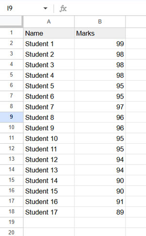
Assume you have student names in column A and their marks in column B. Let’s first filter the max N values using formulas, and then apply filtering using the Google Sheets Data Menu.
Filter Max N Values Using Formulas in Google Sheets
Sample Data:
Formulas and Their Features
| Formula | Purpose |
=SORTN(data, n, 0, 2, FALSE) | Top N (Exactly N, No Extra Ties): Extracts exactly the first N rows from a descending sorted range. |
=SORTN(data, n, 1, 2, FALSE) | Top N + All Duplicates of Nth: Extracts the first N rows from a descending sorted range and includes any additional rows identical to the Nth value. |
=SORTN(data, n, 2, 2, FALSE) | Top N (Distinct Values Only): Extracts the first N unique values from a descending sorted range, ignoring duplicates. |
=SORTN(data, n, 3, 2, FALSE) | Top N (Distinct Values + All Occurrences): Extracts the first N unique values from a descending sorted range and includes all their duplicates. |
Where data is a two-column range (Column A for names, Column B for marks), and n determines the number of top values to extract.
Example 1: Extract Top 3 (Exactly 3, No Extra Ties)
Formula:
=SORTN(A2:B, 3, 0, 2, FALSE)This formula extracts exactly the top 3 highest-scoring students:
| Name | Marks |
| Student 1 | 99 |
| Student 2 | 98 |
| Student 3 | 98 |
Example 2: Extract Top 3 + All Duplicates of 3rd
Formula:
=SORTN(A2:B, 3, 1, 2, FALSE)This formula extracts the top 3 highest scores, including all ties at the 3rd position:
| Name | Marks |
| Student 1 | 99 |
| Student 2 | 98 |
| Student 3 | 98 |
| Student 4 | 98 |
Example 3: Extract Top 3 Distinct Values
Formula:
=SORTN(A2:B, 3, 2, 2, FALSE)This formula extracts the top 3 distinct scores, ignoring duplicate values:
| Name | Marks |
| Student 1 | 99 |
| Student 2 | 98 |
| Student 7 | 97 |
Example 4: Extract Top 3 Distinct Values + All Occurrences
Formula:
=SORTN(A2:B, 3, 3, 2, FALSE)This formula extracts the top 3 distinct values and includes all students with those scores:
| Name | Marks |
| Student 1 | 99 |
| Student 2 | 98 |
| Student 3 | 98 |
| Student 4 | 98 |
| Student 7 | 97 |
How Does This Formula Filter Max N Values?
The SORTN function is designed to extract the top N rows from a sorted range. It offers four tie modes to control whether duplicates are included or excluded.
- We sort the data in descending order based on marks.
- The tie modes (0 to 3) determine how duplicates are handled.
These formulas help you filter the top N in Google Sheets while offering flexibility based on whether you want to include or exclude ties.
Filter Max N Using the Data Menu in Google Sheets
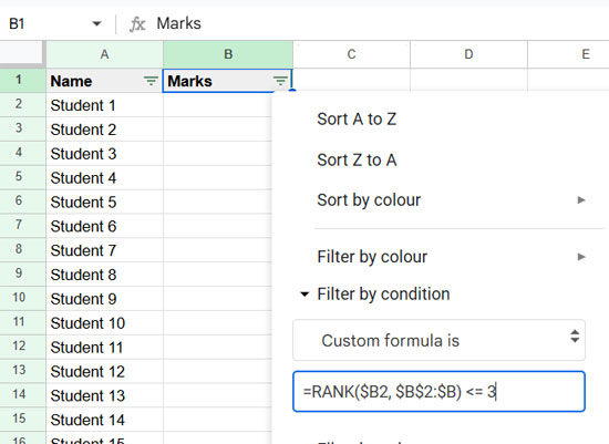
To filter the largest N values using the Data menu, you can apply custom formulas in Google Sheets:
Formula for Top N + All Duplicates of Nth (Example 2 Equivalent)
=RANK(value, data) <= nFormula for Top N Distinct + All Duplicates (Example 4 Equivalent)
=RANK(value, UNIQUE(data)) <= 3Steps to Apply the Filter:
- Select Cell B1 (or the header of your column).
- Click Data > Create a filter.
- Open the filter drop-down in cell B1.
- Click “Filter by Condition”, then select “Custom formula is”.
- Copy-paste one of the formulas above.
- Click OK.
This method will filter the top N values in Google Sheets dynamically, based on your selected formula.
Resources
- How to Find the Highest N Values in Each Group in Google Sheets – Similar to Tie Mode 3.
- Summing the Largest N Values by Group in Google Sheets – Similar to Tie Mode 0.
- Find Max N Values in a Row and Return Headers in Google Sheets – Similar to Tie Mode 1 & 3.
- Find Top N Values with Criteria in Google Sheets (MAX/LARGE) – Covers all four tie modes.
- How to Highlight Largest 3 Values in Each Row in Google Sheets – Applies different tie modes for highlighting.


