I have a sales report in Google Sheets where I want to extract only the top n items based on sales volume. How can I do that?
Let’s explore how to extract the top n items from a table or list in Google Sheets.
In the sample sales report below, columns A to F contain sales data for various landscaping materials.
Sample Data:
| Item | Unit | Qty | Rate | Sales Amount | Project |
| 3/8″ Full Crushed Lime Stone | Ton | 624.42 | 8.00 | 4995.36 | DXB |
| 3/16″ Full Crushed Lime Stone | Ton | 70.12 | 8.00 | 560.96 | DXB |
| Black Washed Sand | Ton | 77.86 | 8.00 | 622.88 | DXB |
| Sub Base | Ton | 631.64 | 8.00 | 5053.12 | ABD |
| Black Sand | Ton | 300.00 | 8.00 | 2400.00 | DXB |
| Cobble Stone 35-80 MM | Ton | 300.00 | 20.00 | 6000.00 | DXB |
| Cobble Stone 40-60 MM | Ton | 149.92 | 20.00 | 2998.40 | DXB |
| River Pebbles | Ton | 7.00 | 232.00 | 1624.00 | ABD |
| Road Base 50 mm Down | Ton | 165.80 | 7.00 | 1160.60 | DXB |
| Limestone 40-80 MM | Ton | 815.36 | 11.00 | 8,968.96 | DXB |
To extract the top 5 items based on sales volume in column C, you can use either the QUERY function or a combination of FILTER and SORTN, depending on your needs:
- QUERY: Suitable for extracting the top n records with the option to add additional criteria.
- FILTER + SORTN: Apply conditions before extracting the top n items plus duplicates, if any. In this case, items with the same sales quantity are considered as a single occurrence (counted as one entity).
Extract Top N Items Using QUERY Function in Google Sheets
In the sample data, we have the sales volume in column C. Assume you want to extract the top 5 records from this dataset, where n is 5.
You can use the following QUERY formula:
=QUERY(A1:F, "SELECT A, B, C, D, E, F ORDER BY C DESC LIMIT 5", 1)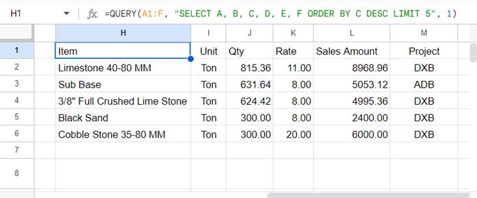
This formula selects columns A to F and sorts column C (Qty) in descending order, so the top items are moved to the top. It limits the output to 5 rows.
The number 1 in the last part indicates the number of header rows in your data range. If your data starts from A2:F, excluding the header in A1:F1, you would specify it as 0.
This formula has one advantage and one disadvantage. The advantage is that you can apply filtering before returning the top 5 items from the range.
For example, you can extract the top 5 items supplied to a specific project, here “DXB”
=QUERY(A1:F, "SELECT A, B, C, D, E, F WHERE F ='DXB' ORDER BY C DESC LIMIT 5", 1)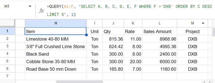
Note: The QUERY function is case-sensitive. Please take care when applying criteria.
The disadvantage is that when there are duplicate values in the column being analyzed for the top n (in this case, Qty), it does not return the top n unique sales volumes.
Here’s where the FILTER and SORTN combo shines.
Extract Top N Items Using FILTER and SORTN Functions in Google Sheets
Do you want to extract the top n unique values and all duplicates of these values, if any? Look no further—the SORTN function is the answer.
The following formula will return the top 5 records from the sales data in A2:F (when using SORTN, exclude the header row):
=SORTN(A2:F, 5, 3, 3, FALSE)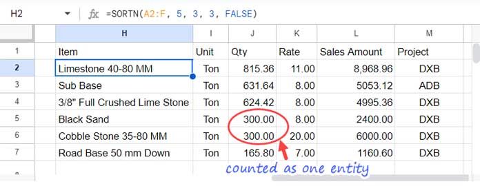
There are 6 records when we expect 5. This is because the quantity 300, which is in the top 5, occurs twice. This means all occurrences of the same top n sales volume will be included.
The formula follows the syntax:
SORTN(range, [n], [display_ties_mode], [sort_column], [is_ascending], [sort_column2, …], [is_ascending2, …])Where:
range: A2:F (the range to extract the top n items)n: 5 (the number of items to extract)display_ties_mode: 3 (mode to extract the top n items plus all duplicates)sort_column: 3 (column index on which to apply the tie mode, here the Qty column)is_ascending: FALSE (to sort the range in descending order based onsort_column)
If you want to apply a condition, use the FILTER function with the range argument.
For example, to extract the top 5 items supplied to the “DXB” project, use the formula below:
=SORTN(FILTER(A2:F, F2:F="DXB"), 5, 3, 3, FALSE)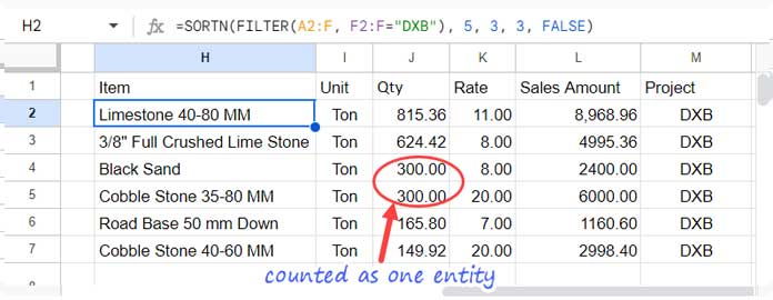
In this, the FILTER function filters A2:F where F2:F="DXB".


Thanks so much!
Is there a way to add a condition to it?
So, for your example, if you had another column titled “product type,” and you wanted the top quantity sales for all sand products?
Hi, Abigail Ryan,
Assume column F contains the “Product Type.”
Here are the formulas based on it.
Query:
=Query(A1:F,"Select A,B,C,D,E where lower(F)='sand' Order by C Desc Limit 5")SORTN:
=sortn(filter(A2:E,F2:F="Sand"),5,0,3,0)Possible to set the limit to be dynamic to a cell reference?
Hi, Brad,
We can do that. In the below example, cell E1 controls the Query Limit clause.
=Query(A1:B,"Select A,sum(B) group by A order by sum(B) desc limit "&E1&" label sum(B)'Sales'")This was great. Exactly what I was looking for.
You saved me a ton of time, thanks!
You should leave the formula in the article.
Hi, Brendan,
Sorry for the inconvenience. I’ll update the post by today itself.