When analyzing data in Google Sheets, you often need to get the top N% scores per group dynamically. This technique is useful for various scenarios, such as:
- Identifying top customers based on purchases
- Analyzing best-selling products within each category
- Selecting top-performing employees or students
- Targeting marketing campaigns at high-value segments
In this guide, we’ll explore how to use Google Sheets functions like FILTER and PERCENTILE to efficiently extract the top N% values per group. We’ll also cover a method to accomplish this without a helper column for a more streamlined approach.
Example: Identifying the Top 20% of Best-Selling Products by Category
Sample Data
We’ll use the following dataset, which contains product names, categories, and units sold:
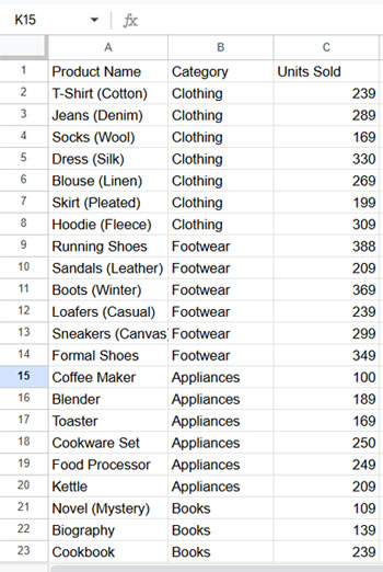
Our goal is to get the top 20% scores per group, meaning we will determine the 80th percentile within each category and include all products that meet or exceed that threshold.
📋 To make it easier to practice, click here to make a copy of the sample Google Sheet and follow along with the steps in real time.
Step 1: Find the Nth Percentile Per Group
To determine the top N% threshold within each group, we use the PERCENTILE function, which finds the value above which the top N% of data points fall.
Formula to Calculate the 80th Percentile Per Group
Enter the following formula in cell D2 and drag it down for all rows:
=PERCENTILE(FILTER($C$2:$C, $B$2:$B=B2), 80%)
How It Works:
FILTER($C$2:$C, $B$2:$B=B2): Extracts only the sales numbers for the current row’s category.PERCENTILE(..., 80%): Returns the 80th percentile (the threshold for the top 20%).- Dragging this formula down ensures each row has the correct percentile value for its category.
After applying this formula, column D will contain the 80th percentile value for each group.
Step 2: Filter Values Greater Than or Equal to the Nth Percentile
Now that we have the percentile threshold for each group, we can filter products that meet or exceed this value.
Formula to Filter the Top N% Values
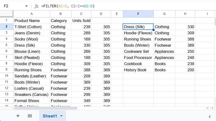
Enter the following formula in cell F2:
=FILTER(A2:C, C2:C>=D2:D)Explanation:
FILTER(A2:C, C2:C>=D2:D):- Filters product names, categories, and units sold (columns A to C).
- Includes only rows where Units Sold (column C) is greater than or equal to the percentile value in column D.
Expected Output
After applying this filter, you will see only the top 20% of products in each category based on sales.
Alternative: Get the Top N% Scores Per Group Without a Helper Column
If you want a more efficient formula that doesn’t require a helper column, you can use the MAP and LAMBDA functions (available in Google Sheets).
Formula to Calculate Percentile On-the-Fly
Clear any previous formulas in column D and enter the following formula in cell D2. There’s no need to drag it down, as it automatically expands to cover all rows.
=MAP(B2:B, LAMBDA(row, PERCENTILE(FILTER($C$2:$C, $B$2:$B=row), 80%)))How It Works:
MAP(B2:B, LAMBDA(row, ...)): Iterates over each row’s category.FILTER($C$2:$C, $B$2:$B=row): Extracts sales for that category.PERCENTILE(..., 80%): Finds the 80th percentile for that category.
Directly Use This in FILTER Formula
Instead of using a separate helper column, you can embed this formula directly inside the FILTER function:
=FILTER(A2:C, C2:C >= MAP(B2:B, LAMBDA(row, PERCENTILE(FILTER($C$2:$C, $B$2:$B=row), 80%))))Why This Method Is Better
This approach eliminates the need for extra columns, making your spreadsheet cleaner and more efficient. The formula is more streamlined, reducing manual work and improving readability. Additionally, it dynamically adjusts for all groups, ensuring accurate percentile calculations without requiring modifications for different datasets.
Conclusion
By following these methods, you can efficiently get the top N% scores per group in Google Sheets. Whether you choose to use a helper column or an inline formula, both approaches allow you to dynamically filter and analyze top-performing values.
This technique is highly versatile and can be applied to:
- Sales analysis (top-selling products per category)
- Marketing insights (top-spending customers per segment)
- Education tracking (top-scoring students per subject)
By leveraging the FILTER and PERCENTILE functions, you can automate complex data filtering in Google Sheets with ease!
Additional Resources
For further learning, check out these related guides:
- Percentile Rank Conditional Formatting in Google Sheets
- Calculating Percentile for Each Group in Google Sheets
- How to Use Percentage in IF Statements in Google Sheets
- How to Randomly Extract a Certain Percentage of Rows
- Average of Top N Percent of Values – With or Without Conditions
- How to Calculate Reverse Percentage in Google Sheets


