VLOOKUP with date ranges in Google Sheets can be more intricate than a single approach. There are two approaches, and both are quite interesting.
In the first approach, there are two criteria: searching for a date (exact or less than the specified date) in one column and a text in another column, returning a value from a third column. This is useful when you want to find positions, availability, etc., on a particular date.
The second approach involves looking up a date in the start and end date columns and returning a value from another column. We have already discussed this approach in detail in the article “Lookup a Date Between Two Dates in Google Sheets“.
Here, “VLOOKUP in a date range” refers to our first approach. Let’s proceed to that example.
Sample Data
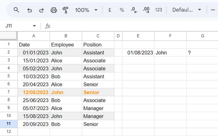
The table consists of three columns in A1:C, where A1:A contains dates, B1:B contains employee names, and C1:C contains their current positions.
Each employee may appear multiple times in column B if they’ve been promoted. The dates in column A represent when the promotion occurred. The positions in column C indicate the current position of the employee at the given date.
We want to look up a date and employee name in columns A and B and return their current position. Let’s see how to use VLOOKUP in a date range in Google Sheets for this.
VLOOKUP for a Date Range: Logic in Google Sheets
Cell E2 contains the date 01/08/2023, and F2 contains the employee name “John”. We want to find John’s position on 01/08/2023.
The VLOOKUP function is capable of searching only one column, not two. Thus, we need to meet this requirement when using VLOOKUP.
To accomplish this, we’ll use VLOOKUP to search for the date, not the name. How?
First, we’ll first filter the table to include only rows where the employee name is “John” using the FILTER function. Then, we’ll sort this filtered data and apply the VLOOKUP function to search for the date in this filtered table.
Ensure that the first column contains dates, as VLOOKUP searches the first column in the range.
This is the logic behind using VLOOKUP for a date range.
Step-by-Step Instructions
The following formula filters the table, the range A:C, based on the name in cell F2:
=FILTER(A:C, B:B=F2)Syntax: FILTER(range, condition1, [condition2, …])
In the above formula, the range is A:C, and condition1 is B:B=F2. It’s that simple.
To sort it in ascending order by the date column, use:
=SORT(FILTER(A:C, B:B=F2))Now, let’s examine the VLOOKUP syntax: VLOOKUP(search_key, range, index, [is_sorted])
The search_key is the date in cell E2, and the range is the above filter formula. Since we need to return the position from the third column, specify 3 as the index.
You can leave the last parameter, which is is_sorted, or specify TRUE
=VLOOKUP(E2, SORT(FILTER(A:C, B:B=F2)), 3, TRUE)This way, we can use VLOOKUP for a date range in Google Sheets.
Handling Multiple Search Keys in VLOOKUP Date Range Formulas
You can use the above formula to:
- Find the position of one employee on a given date
- Find the positions of one employee on multiple given dates
- Find the positions of multiple employees on a given date
- Find the positions of multiple employees on multiple given dates
The formula will remain the same if you prefer to drag and drop or use a lambda approach.
Here is how to handle multiple search keys in VLOOKUP date ranges in Google Sheets.
In the following example, I want to look up the dates in E2:E4 (the dates can be the same or different for each name) and names in F2:F4 within the range A:C.
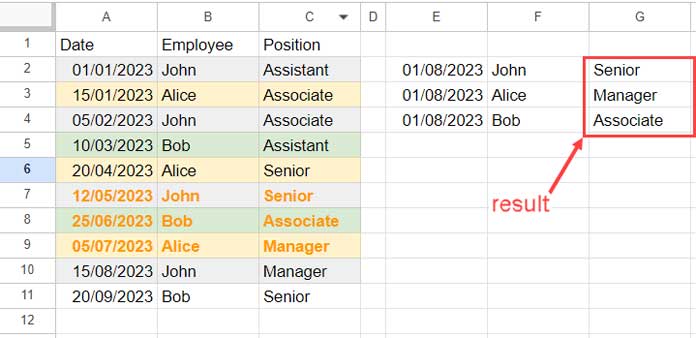
Option 1:
Enter the earlier VLOOKUP in cell G2 and drag the fill handle on the bottom right corner to G4.
Option 2:
Empty the range G2:G4 and use the following array formula in cell G2:
=MAP(E2:E4, F2:F4, LAMBDA(x, y, VLOOKUP(x, SORT(FILTER(A:C, B:B=y)), 3)))This formula iterates through each pair of dates and employee names in E2:E4 and F2:F4 respectively, performing a VLOOKUP for each combination to retrieve the corresponding position from the sorted and filtered range A:C.
Resources
- Lookup Dates and Return Currency Rates in an Array in Google Sheets
- Lookup Earliest Dates in Google Sheets in a List of Items
- How to Lookup Latest Dates in Google Sheets
- Vlookup Date in Timestamp Column in Google Sheets
- Conditionally Lookup Dates in Date Range in Google Sheets
- XLOOKUP with Date and Time in Google Sheets


Hi Prashanth,
Could you please assist me with my problem? I have a reference table (A1:C8) consisting of doctors with their ranks, which may differ according to date and time. Then I have a table (H2:J) to be automatically filled with a formula (J2:J), based on certain dates. For example, Dr. Imelda’s rank on April 4, 2024, was DU01, but on May 10, 2024, her rank is DU02. Thank you very much.
For the table with columns Date, Doctor, and Rank in A1:C, and for the criteria to lookup, i.e., Date in H2:H and Doctor in I2:I, you can use the below formula in J2:
=MAP(H2:H, I2:I, LAMBDA(x, y, CHOOSECOLS(SORTN(FILTER(A:C, B:B=y, A:A<=x), 1, 0, 1, FALSE), 3)))Thank you very much Mr. Prashanth for the explaination! Very clear.
Thanks for this post.
The formula only checks the start date, looking for the closest Start Date.
But what if the reference date is greater than the End Date?
For 17/2/18, it works, but what about 1/3/18?
It will return the same result even if 1/3/18 is not in the range 16/2/18 – 28/2/18. Thanks
Hi, David Leal,
You can sort out that issue by modifying the Vlookup range as below.
=ifna(VLOOKUP(F2,{A2:D;{max(B2:B)+1,"","",""}},4,1))Here is an alternative Filter solution.
=ifna(filter(D2:D,(GTE(F2,A2:A)*LTE(F2,B2:B))))I’ve been banging my head against a challenge for a while. It is the closest approach I’ve found so far, but it goes a step further.
Could you possibly help?
I need a formula that does the following:
1. Loo up the value of A2 in column D. There are multiple matches.
2. Of the rows matched in step 1, Lookup the value of B2 in column E.
3. Of the rows matched in step 2, Lookup the date range for C2 in column F as you’ve accomplished in the formula in this tutorial.
Please help if you can!
Thank you,
Peter
Hi, Peter Beddow,
I will try if you share an editable sheet that contains-
1. Limited sample data.
2. Your expected result (hand-entered).
Feel free to use the “Reply” below. I won’t publish the Sheet/URL.
Hi Paul,
I tried all your formulas and want to use the last one, because it seems to be the solution for my table.
But I receive an error message for the “sort” function in the formula: “that function isn’t valid” 🙁
Did you have any idea?
Many thanks
Regards
Kei
Hi, Kei,
SORT is a valid Google Sheets function. If you can share a copy of the sheet that you are working on (or a sample with demo data), I may be able to assist you.
Hi Prashanth.
I like the approach use here
=ArrayFormula(LOOKUP(2,1/($A$2:$A=F2),$D$2:$D))Would it be impossible to use ArrayFormula?
Hi, Paul,
Already provided within the tutorial 🙂