To look up dates and return currency exchange rates from Google Finance, we can use a combination formula in Google Sheets. This array formula involves the GOOGLEFINANCE, QUERY, and VLOOKUP functions, allowing us to retrieve single or multiple currency rates.

Google Finance provides international exchange rates, along with real-time market quotes and other financial data.

Please refer to the screenshot below. In it, you can see various dates in column A and their corresponding exchange rates in column B.

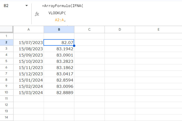
The conversion rate shown is from USD to INR, but you can choose your preferred currencies. There is an array formula in cell B2 that returns these exchange rates. Let’s now dive into the formula and its explanation.

Lookup Dates and Return Currency Rates: Formula and Overview

Here is the formula used in cell B2 to look up dates in A2:A and return currency exchange rates from Google Finance in B2:B:

=ArrayFormula(IFNA(VLOOKUP(
   A2:A, 
   QUERY(
      GOOGLEFINANCE(
         "CURRENCY:USDINR", "PRICE", MIN(A2:A)-5, MAX(A2:A)+5, "DAILY"
      ), 
      "SELECT TODATE(Col1), Col2", 1
   ), 2, 0
)))

When using this formula, replace A2:A with your specific date range reference and USDINR with your required currency codes.

The currency conversion is from USD to INR. To find other currency codes, please check out https://en.wikipedia.org/wiki/ISO_4217.

It’s also important to note the dates specified. Make sure they are not too distant; dates spanning several years may cause issues. Dates within 2 to 3 years are acceptable. Otherwise, the formula may fail or slow down. You will understand the reason in the formula explanation below.

Here is the role of each function in the formula for looking up dates and returning exchange rates.

Formula Explanation

There are three key functions in use: GOOGLEFINANCE, QUERY, and VLOOKUP. Here are their roles:

Part 1: GOOGLEFINANCE

GOOGLEFINANCE("CURRENCY:USDINR", "PRICE", MIN(A2:A)-5, MAX(A2:A)+5, "DAILY")

This formula fetches daily currency exchange rates from the Google Finance website, covering a range from the minimum date minus 5 days to the maximum date plus 5 days specified in column A.

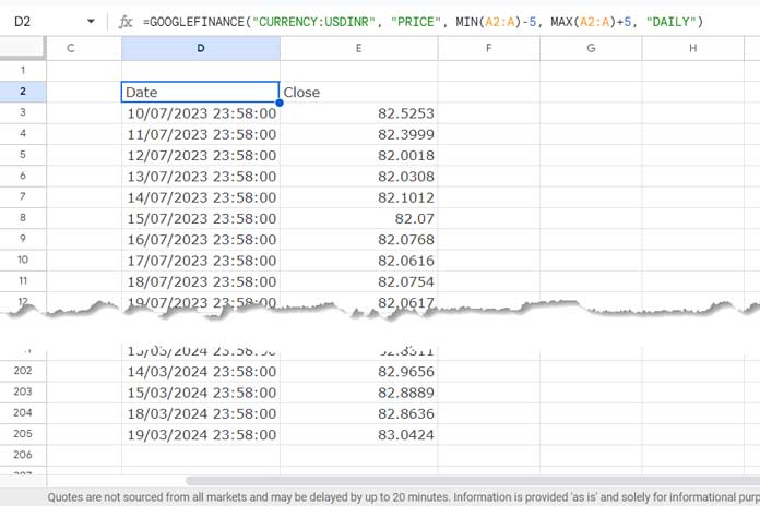
For example, with the sample data, the minimum date is 15/07/2023, and the maximum date is 15/03/2024. Therefore, the formula retrieves currency exchange rates from 10/07/2023 to 20/03/2024. The additional width ensures that we capture all the required information, as GOOGLEFINANCE may sometimes skip some dates at the beginning and end.

The formula returns a two-column array with timestamps in one column and exchange rates in the other. The number of rows in this data will depend on the minimum and maximum dates in column A. Therefore, using distant dates that span several years may slow down performance.

Since we cannot look up dates directly in the timestamp column, we need to convert the timestamps to dates. The following QUERY handles that.

Part 2: QUERY

QUERY(…,"SELECT TODATE(Col1), Col2", 1)

The SELECT clause selects the columns to return; in this case, it’s column 1 and column 2. The TODATE scalar function converts the timestamps in column 1 to dates, so the output will be a date column and a currency exchange rate column.

Part 3: VLOOKUP

VLOOKUP(A2:A, …, 2, 0)

The VLOOKUP function searches for the dates in A2:A within the first column of the QUERY result and returns the exchange rates from the second column.

This way, we can look up dates and return currency exchange rates in Google Sheets.

Resources

• Currency Conversion in Google Sheets Using GOOGLEFINANCE
• Finding Max and Min Values in GoogleFinance Historical Data in Sheets