In various scenarios, you can use conditional lookup to find a date within a start and end date range. We’ll see how to do this in Google Sheets.

For example, you might want to offer a discount based on the travel date to specific cities. In this case, the lookup criteria will be the city name and travel date.

Assume you have a table that lists cities and the discount allowed during specific periods, in the format: city (column 1), start date (column 2), end date (column 3), and discount (column 4).

In this scenario, you can apply conditional lookup to find a city and date within the specified date ranges in the table.

The condition will be the city name (first column), and you want to look up the date in the start (second column) and end date (third column) range to return the appropriate discount (fourth column).

Download Sample Sheet

Step 1: Lookup Date in a Start and End Date Range

Enter the following formula in cell I3 to evaluate whether the date in H3 falls in the range C3:D3:

=ISBETWEEN(H3, C3, D3)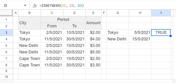

Syntax:

ISBETWEEN(value_to_compare, lower_value, upper_value, [lower_value_is_inclusive], [upper_value_is_inclusive])

Where:

• value_to_compare: H3
• lower_value: C3
• upper_value: D3

Step 2: Lookup Date in Multiple Start and End Dates

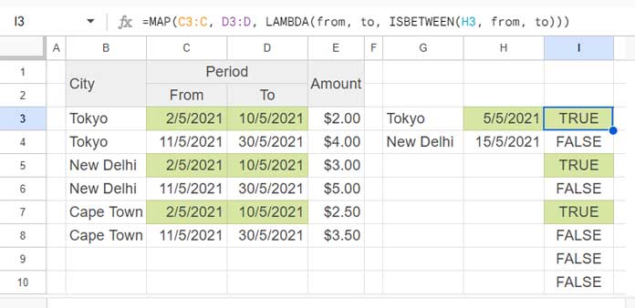
We need to expand this to columns C3:C (lower_value) and D3:D (upper_value) so that it can evaluate whether the date in H3 falls between any date ranges in columns C and D.

To do that, we will use the MAP Lambda function.

Syntax:

MAP(array1, [array2, …],LAMBDA([name, …], formula_expression))

We want the ISBETWEEN function to apply to each row in the range C3:D. So array1 and array2 will be C3:C and D3:D respectively.

MAP(C3:C, D3:D, LAMBDA([name, …], formula_expression))

The formula_expression will be our step 1 formula:

MAP(C3:C, D3:D, LAMBDA([name, …], ISBETWEEN(H3, C3, D3)))

Assign names to C3 and D3 within the LAMBDA so MAP will map these elements in each row in the arrays.

=MAP(C3:C, D3:D, LAMBDA(from, to, ISBETWEEN(H3, from, to)))

This is the important step to conditionally look up a date in the start and end date range.

Step 3: Conditionally Lookup Dates in Start-End Ranges

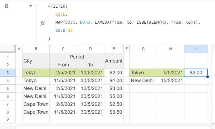
We can now use the FILTER function to filter the range E3:E where the above formula returns TRUE and the city in G3 matches B3:B.

Syntax:

FILTER(range, condition1, [condition2, …])

Formula:

=FILTER(
   E3:E, 
   MAP(C3:C, D3:D, LAMBDA(from, to, ISBETWEEN(H3, from, to))), 
   B3:B=G3
)

Where:

• range: E3:E
• condition1: MAP(C3:C, D3:D, LAMBDA(from, to, ISBETWEEN(H3, from, to)))
• condition2: B3:B=G3

We have conditionally looked up the date in H3 within the range C3:D, the city in G3 within B3:B, and returned the corresponding value from E3:E.

Step 4: Conditionally Lookup Multiple Dates in Start-End Ranges

In the above formula, we used the search keys in G3 (city) and H3 (lookup_date).

You can use another MAP with the above formula to expand G3 and H3 to G3:H.

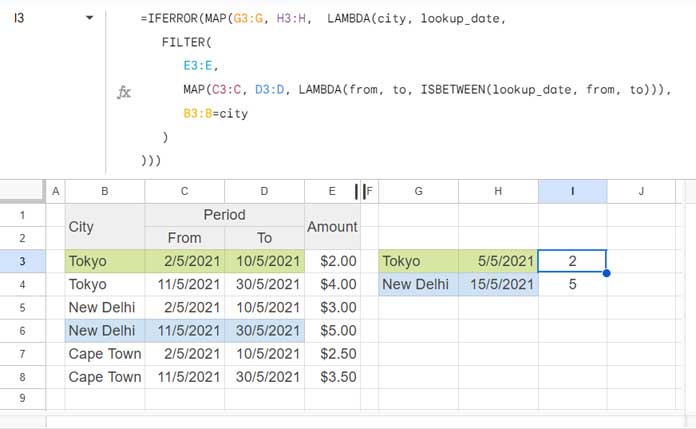
In that MAP, array1 will be G3:G and array2 will be H3:H, and the formula_expression will be the above step 3 formula. In that, we will replace G3 with city and H3 with lookup_date, two assigned names.

=MAP(G3:G, H3:H,  LAMBDA(city, lookup_date, 
   FILTER(
      E3:E, 
      MAP(C3:C, D3:D, LAMBDA(from, to, ISBETWEEN(lookup_date, from, to))), 
      B3:B=city
   )
))

This will return errors in empty rows. So it’s advisable to wrap it with the IFERROR function:

=IFERROR(MAP(G3:G, H3:H,  LAMBDA(city, lookup_date, 
   FILTER(
      E3:E, 
      MAP(C3:C, D3:D, LAMBDA(from, to, ISBETWEEN(lookup_date, from, to))), 
      B3:B=city
   )
)))

Resources

• Lookup a Date Between Two Dates in Google Sheets
• How to Vlookup a Date Range in Google Sheets