Lookup the latest date is not simply about finding the maximum date in a column; it is a broader topic in Google Sheets. It allows you to get a value based on the most recent date or look up a search key in the latest entry row. For this, you can use the XLOOKUP function in Google Sheets.

I prefer XLOOKUP over VLOOKUP (both are lookup functions with vertical lookup capability in unsorted data) because of its ability to lookup any column in a range. VLOOKUP is limited to looking up in the first column.

Lookup the Latest Date in a Column in Google Sheets

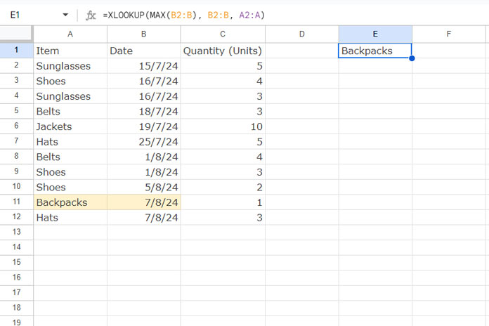
Assume you have various items in one column and their receipt dates in another column. To find the item received on the most recent date, you can use the following formulas.

In this example, I consider the dates in column B and items in column A starting from row #2, as row #1 is for titles.

=XLOOKUP(MAX(B2:B), B2:B, A2:A)

This formula looks up the latest date returned by the MAX function from top to bottom in the range B2:B and returns the corresponding value from A2:A.

To lookup the latest date from the bottom of a range to the top, you may use the following XLOOKUP formula:

=XLOOKUP(MAX(B2:B), B2:B, A2:A,,,-1)

Both formulas will get the same result if there are no multiple occurrences of the max date in the column.

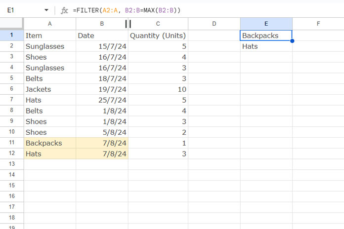
To get all occurrences, you should rather depend on the FILTER formula as XLOOKUP is not suitable in this case:

=FILTER(A2:A, B2:B=MAX(B2:B))

The FILTER function filters the range A2:A where the range B2:B matches the max date in B2:B.

Lookup a Search Key in a Column in the Latest Date Row

This is a different scenario. Assume you want to lookup when you last received an item as well as its quantity. Here we should adopt a different approach.

The following formula looks up “Sunglasses” in A2:A and returns the latest receipt date from B2:B.

=XLOOKUP("Sunglasses", SORT(A2:A, B2:B, FALSE), SORT(B2:B, 1, FALSE))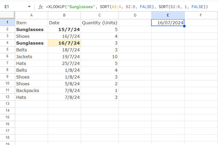

In this, the search key is “Sunglasses.”

How does this formula lookup this key in the latest date row?

I have sorted the search key column, i.e., A2:A, based on the date in descending order and the result column, i.e., the dates, also in descending order.

• SORT(A2:A, B2:B, FALSE) – sorts A2:A based on B2:B in descending order
• SORT(B2:B, 1, FALSE) – sorts B2:B in descending order.

The result will be a date value. Navigate to the result cell and apply Format > Number > Date.

Note for Excel users: This formula may not work in Excel; you may use SORTBY instead of SORT for the search key (lookup) column sorting.

If you want to lookup the search key “Sunglasses” and return its latest delivery quantity, you should use the formula as follows:

=XLOOKUP("Sunglasses", SORT(A2:A, B2:B, FALSE), SORT(C2:C, B2:B, FALSE))

Where:

• Search Key: “Sunglasses”
• Lookup Range: SORT(A2:A, B2:B, FALSE) – sorts items based on dates in descending order
• Result Range: SORT(C2:C, B2:B, FALSE) – sorts quantities based on dates in descending order

When you have the same item received multiple times, you should use FILTER instead:

=FILTER(A2:C, A2:A="Sunglasses", B2:B=MAX(IF(A2:A="Sunglasses", B2:B,)))

The FILTER function filters the range A2:C where A2:A is equal to “Sunglasses” and B2:B is equal to the max date in the date range, ensuring that only the latest entry is included.

Resources

• Lookup Latest Value in Excel and Google Sheets
• Extract the Earliest or Latest Record in Each Category in Google Sheets
• Formula to Combine Rows and Get Latest Values in Google Sheets
• Highlight the Latest Value Change Rows in Google Sheets
• How to Highlight the Latest N Values in Google Sheets
• Get the Latest Non-Blank Value by Date in Google Sheets