It’s a must to learn how to lookup earliest dates in Google Sheets. It’s useful in different sectors and most prominently in logistics.
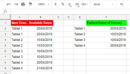
The date has an important role in every part of our life. Please scroll down and see the image to understand about lookup earliest dates that I’m talking about.
There are countless examples where you may want to lookup earliest dates. If you are working as a logistics coordinator, handling material purchases, or if you are selling products through online marketplaces you may want to lookup earliest dates.
For example, if you have ordered an item that may come in different lots on different days, you can use the below tips.
Just enter the schedule of arrival of all such items and use my lookup tips to find the earliest arrival date. So that you can make the necessary arrangements to receive the material.
Then How to Lookup Earliest Dates in Google Sheets?
No need to go through all the dates manually in a list to find the earliest dates in Google Sheets. I am going to make your this type of job much easier by providing you a Google Sheets formula to solve this. I know this is one of the most commonly occurring office task.
See this image first and understand what you are going to learn.

When you have different items (Column A) and different delivery dates (Column B) you may want to find an Array Formula that can return multiple earliest dates in Google Sheets.
If it’s a single item in Column A and multiple delivery dates, you can use Google Sheets MIN or SMALL functions. You can follow the below link to learn about that simple tips.
Similar: Find Minimum Value and Return Value from Another Column
But in our above example, we can use the Vlookup function in Array Form. But there is a twist. The lookup range in Vlookup will be a combination of SORT and SORTN formulas.
See my list of items in column A and possible delivery dates in Column B. In Column F with the help of my formula, I could find the earliest delivery dates of each items.
Formula to Lookup Earliest Dates in Google Sheets
The following is my formula in Cell F2 in the above example.
=ArrayFormula(VLOOKUP(E2:E5,SORTN(SORT(A2:B9,2,TRUE,1,TRUE),20,2,1,TRUE),2,FALSE))
Actually the highlighted (Cyan and Pale Green) part of the formula is enough. I’ll explain it later.

This formula to lookup earliest dates in Google Sheets is a combination of SORT, SORTN formulas. This combo acts as a lookup range in Vlookup.
Formula Logic and Explanation
The order of the formula is like this. SORT > SORTN > VLOOKUP. That means first you should learn the use of SORT, then SORTN that followed by Vlookup.
So let me explain the role of each of the above mentioned functions in the formula to Lookup earliest dates in Google Sheets.
SORT
=SORT(A2:B9,2,TRUE,1,TRUE)
Syntax:
SORT(range, sort_column, is_ascending, [sort_column2, ...], [is_ascending2, ...])
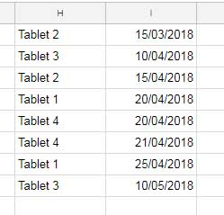
Here I’ve just sorted our sample data, that first based on column 2 that is the column with dates in ascending order then by column 1 that also in ascending order.
In this sorting, all the lowest dates comes to the top of the row.

Now the next step is to delete the duplicates in Column 1. For that, we can use SORTN, an advanced Sort function in Google Sheets.
To learn more about this function please refer my Google Sheets Functions Guide.
SORTN
=SORTN(SORT(A2:B9,2,TRUE,1,TRUE),20,2,1,TRUE)
Syntax:
SORTN(range, [n], [display_ties_mode], [sort_column], [is_ascending], [sort_column2, ...], [is_ascending2, ...])
Please refer to the above first screenshot. There you can see that the duplicate values are in the first column. Now take a look at the arguments used in the formula.
RANGE:
SORT(A2:B9,2,TRUE,1,TRUE)
[N] = 20
This’s the number of rows to be returned by the formula. I’ve just put a random number in this example because I know the returned rows after deleting the duplicates would be less than 20.
When you have a large number of rows and you are unsure about the rows you can use 9^9 instead of putting 20 or any other number.
You May Like: Remove Duplicates in Google Sheets [The Complete Guide and Sample Sheet]
DISPLAY_TIES_MODE: To remove duplicates, you should use the number 2 as display_ties_mode in SORTN (I’ve detailed more about this in my relevant SORTN tutorial.
SORT_COLUMN: It’s the column to sort. That means you should put the column number that contains the duplicates and here it’s Column 1.
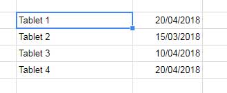
Here is the output.

Actually, this formula itself is enough to Lookup Earliest Dates in Google Sheets in a List of Items. The Vlookup part in our master formula is optional.
VLOOKUP
If you want to find the earliest delivery of items of your choice, you can use Vlookup on the just above result.
The above SORTN formula returns all the items and its earliest delivery dates.
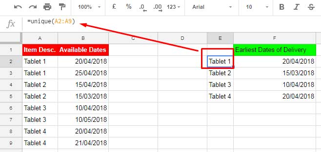
First, in a column type the item names of which you want to get the earliest delivery dates.
Here I am using all the items. So I’ve used a Unique formula to return the unique items in Column E.

This’s our master formula which I’ve already shared in the beginning of this tutorial.
=ArrayFormula(VLOOKUP(E2:E5,SORTN(SORT(A2:B9,2,TRUE,1,TRUE),20,2,1,TRUE),2,FALSE))
See the Vlookup Syntax
VLOOKUP(search_key, range, index, [is_sorted])
In this formula, the search key is in E2: E5. The range is replaced by the above SORTN+SORT combo range. When you have to lookup multiple search keys in Vlookup, you should use the ArrayFormula in Vlookup.
Must Read: How to Use Vlookup to Return An Array Result in Google Sheets
That’s all. The above is the easiest way to lookup earliest dates in Google Sheets in a list of items.


This worked like magic. Thanks so much 🙂