Lookup a Date Between Two Dates in Google Sheets

The lookup functions are designed to search for a key in a single column or row, not in two columns or rows. However, when it comes to searching for a date between two dates, it requires two search key columns. Let’s explore how to accomplish this in Google Sheets.

Sample Data

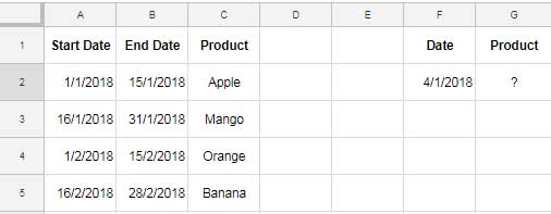
The sample data consists of the Start Date, End Date, and Product in columns A to C.

We want to look up a date between the start and end dates in each row of the range and return the product name.

Sample data for looking up a date between two dates in Google Sheets

In Google Sheets, we will see how to use VLOOKUP and XLOOKUP functions to lookup a date between two dates (start and end dates) in each row.

VLOOKUP a Date in Start and End Date Columns

We understand that VLOOKUP can’t search in two columns simultaneously. Therefore, we must merge the start and end date columns into a single column using the following logic.

We want to search for the date 04/01/2018, entered in cell F2, within the start and end dates in columns A2:B. Here are the step-by-step instructions:

The following formula will merge columns A2:A and B2:B into a single column containing 1s and 0s, where 1 represents a match with the search key, and 0 for no match.

=ArrayFormula((A2:A<=F2)*(B2:B>=F2))

Note: The Explanation has been added after a few paragraphs below.

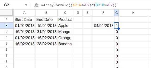
Combined start and end date column for lookup

This merged column will serve as the VLOOKUP search column, which will be the first column in the lookup range.

We want to return values from column C. Therefore, we combine C2:C with this search column using HSTACK as follows.

=HSTACK(ArrayFormula((A2:A<=F2)*(B2:B>=F2)), C2:C)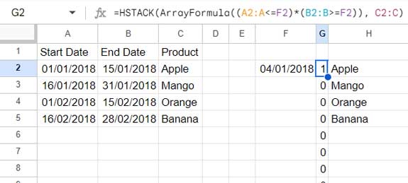

Combining merged date columns and result column for lookup range

This combined array will be used as the range parameter in the VLOOKUP.

Syntax: VLOOKUP(search_key, range, index, [is_sorted])

Since this range contains 1s or 0s in the first column, where 1 represents a match, we set the search_key as 1. The index column will be 2 because the product column is the second column in this range.

So the formula will be:

=VLOOKUP(1, HSTACK(ArrayFormula((A2:A<=F2)*(B2:B>=F2)), C2:C), 2, FALSE)

Explanation:

=ArrayFormula((A2:A<=F2)*(B2:B>=F2))

This array formula evaluates each cell in the range A2:A to check if it’s less than or equal to the date in cell F2 (the lookup date). Similarly, it checks each cell in the range B2:B to see if it’s greater than or equal to the lookup date.

The multiplication operation (*) combines the results of these comparisons, producing a resulting array where each element is either 1 (if the condition is true) or 0 (if the condition is false).

Therefore, the resulting array effectively indicates whether the lookup date falls within the range defined by the start and end dates in columns A and B respectively.

XLOOKUP a Date in Start and End Date Columns

Another method to search for a date between two dates is using XLOOKUP.

The formula follows the same logic as described above. The only difference is that we should specify the search and result columns separately in the formula. There is no need to combine them using HSTACK as previously done. The search key will be 1, and the index column is not required.

Syntax: XLOOKUP(search_key, lookup_range, result_range, [missing_value], [match_mode], [search_mode])

Formula:

=XLOOKUP(1, ArrayFormula((A2:A<=F2)*(B2:B>=F2)), C2:C)

Where:

search_key: 1
lookup_range: ArrayFormula((A2:A<=F2)*(B2:B>=F2))
result_range: C2:C

Using Multiple Search Keys in Start and End Date Columns

In the above example, we have a single search date in cell F2.

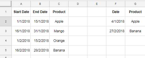
But what if you want to look up the dates in the range F2:F3 within columns A2:A and B2:B, and return the corresponding products from column C2:C?

Example of looking up dates between start and end dates

Simply including F2:F3 directly in the formulas won’t provide the desired result. Instead, you may utilize the MAP lambda function.

Syntax: MAP(array1, [array2, …], lambda)

In this case, we’ll use F2:F3 as array1. There is no need for array2. The lambda function will be the VLOOKUP or XLOOKUP formula mentioned previously.

VLOOKUP Multiple Dates in Start and End Date Columns

=MAP(F2:F3, LAMBDA(value, VLOOKUP(1, HSTACK(ArrayFormula((A2:A<=value)*(B2:B>=value)), C2:C), 2, FALSE)))

XLOOKUP Multiple Dates in Start and End Date Columns

=MAP(F2:F3, LAMBDA(value, XLOOKUP(1, ArrayFormula((A2:A<=value)*(B2:B>=value)), C2:C)))

It’s important to note that using MAP with a large dataset may lead to performance issues.

Resources

Here are some related resources regarding looking up dates within a range in Google Sheets.

29 COMMENTS

R. Krishna December 14, 2022 At 9:50 pm

Hi Prashanth,

Will this formula work with HLOOKUP?

Thanks.

- Prashanth December 15, 2022 At 9:55 am
  
  Hi, R. Krishna,
  
  We can use the latest function bundle (Lambda and helper functions) to create a much cleaner formula.
  
  You may not require the HLOOKUP.
  
  Please explain the problem in detail.
  
stephen Bessette October 21, 2021 At 12:56 am

Hi, I have a sheet with the following.

A1 – Customer name
B1 – Date of first contact
C1 – Date of agreement
S1:BB1 – The month of the year (it runs 36 months across)

When we meet a customer, we enter A1 and B1. When they sign, that is C1.

Then when we bill them, we place a dollar value in the appropriate cell for that month’s revenue (S2:BB2).

The goal is to calculate how many days it was between the “Date of first contact” (column B) and the date of the first payment (Columns S:BB).

- Prashanth October 24, 2021 At 9:15 am
  
  Hi, Stephen Bessette,
  
  In cell D2 enter the below formula to get the month (S1:BB1) correspond to the first non-blank value in that row.
  
  =index($S$1:$BB$1,MATCH(FALSE,ISBLANK(S2:BB2),0))
  
  Drag this formula down the column.
  
  Now you may be able to find the number of days in another column. For that, empty E2:E and enter the below formula in cell E2.
  
  =ArrayFormula(if(len(B2:B),days(D2:D,B2:B),))
  
  This formula will expand down.
  
  If you want, you can replace the above first formula with an array formula.
  
  Empty D2:D and enter the following formula in cell D2.
  
  =index(sortn(query(split(flatten(ROW(S2:BB100)&"|"&S1:BB1&"|"&S2:BB100),"|"), "Select * where Col3 is not null"),9^9,2,1,1),0,2)
  
  This formula has a draw-back. You must have a dollar value in each row.
  
  I’ll try to explain the above formula in my upcoming tutorial.
  
Eva June 2, 2021 At 8:41 am

Hi,

This article is so inspirational – thank you!

I want to pull such data from a start-end dates range in one sheet into a calendar-shaped sheet in the same workbook (there is one cell for each day to count all the instances in which we have bookings for that day but I cannot fix the formula yet). I need a simple formula to insert for each day of the month in the calendar sheet to calculate the number of bookings from the range from-to on the first sheet – is this possible?

Kind regards

- Prashanth June 3, 2021 At 11:28 am
  
  Hi, Eva,
  
  I can try if you could share a mockup/sample of your sheet. Use the “Reply” below to share the URL (I’ll keep that comment private/[won’t publish]).
  
CC March 16, 2021 At 3:50 am

Hello, I have tried the following but have gotten the error of “Function ARRAY_ROW parameter 2 has mismatched row size. Expected: 1095. Actual: 1093”.

Could you help with this formula? Does it work for multiple years?

=ArrayFormula(IF(LEN(E2:E),(VLOOKUP(E2:E,{row(indirect("A"&A2):indirect("A"&B13)),transpose(split(join("",(rept(C2:C13&"|",(B2:B13-A2:A13)+1))),"|"))},2,FALSE)),))

Start Date | End Date | Quarter
8/1/19 | 10/31/19 | Q1 2020
11/1/19 | 1/31/20 | Q2 2020
2/1/20 | 4/30/20 | Q3 2020
5/1/20 | 7/30/20 | Q4 2020
8/1/20 | 10/31/20 | Q1 2021
11/1/20 | 1/31/21 | Q2 2021
2/1/21 | 4/30/21 | Q3 2021
5/1/21 | 7/30/21 | Q4 2021
8/1/21 | 10/31/21 | Q1 2022
11/1/21 | 1/31/22 | Q2 2022
2/1/22 | 4/30/22 | Q3 2022
5/1/22 | 7/30/22 | Q4 2022

- Prashanth March 16, 2021 At 11:21 am
  
  Hi, CC,
  
  It’s because of the three “End Dates” 07/30/20, 07/30/21, and 07/30/22. It should be 07/31/20, 07/31/21, and 07/31/22. If you change that, the formula will work.
  
  But please note that there is one more solution. In the last paragraph, I have linked to another tutorial that has a much simpler solution.
  
  =ArrayFormula(IFERROR(VLOOKUP(E2:E,A2:C,3,1)))
  
  The above Vlookup only requires sequential dates. The above date issue won’t affect it.
  
Anthony February 2, 2021 At 9:25 am

Hi Prashanth,

I’m still pretty new to Google Sheets, but I’m enjoying myself.

I’m afraid I don’t understand the second thing about your master formula.

You have an IF formula where the condition is LEN(, but if I understand LEN correctly, this will just generate a number, something like 42 for example.

How can an IF formula work when a condition is just a number? That is, what is IF doing when I write =IF(42,"True","False")?

I hope my question is clear.

- Prashanth February 2, 2021 At 3:05 pm
  
  Hi, Anthony,
  
  I understand the purpose of LEN is clear to you. It is just to return the number of characters in a cell.
  
  But when we use it with IF, the purpose is different.
  
  Example.
  
  =if(len(A1),"Fruits","Vegetables")
  
  It means if A1 has any value (or A1 has length), return “Fruits”, else “Vegetables”.
  
  It’s an alternative of =if(isblank(A1),"Vegetables","Fruits") or =if(not(isblank(A1)),"Fruits","Vegetables")
  
Adam Housley August 26, 2020 At 6:34 am

First, I’m in a bit over my head, but your formula is the best explanation I’ve read, but I’m still struggling.

In the sheet below (link removed by admin), I need a formula for tab 1, Column E that will return the webinar date (tab 2, Column A) based on the submitted date (tab 1, Column A).

Basically, if the submitted date falls between the dates in tab 2 column C & D, then return the corresponding date listed in tab 2 Column A.

Does that make sense?

- Prashanth August 26, 2020 At 2:53 pm
  
  Hi, Adam Housley,
  
  You can try the below Vlookup Date Range formula.
  
  =ArrayFormula(IFNA(vlookup(A2:A,sort({'Info Zoom Formulas'!C2:D,'Info Zoom Formulas'!A2:A}),3,1)))
  
  This formula to be keyed in E2. It will expand to the rows down. Also covered the entire rows in both the sheets.
  
  Note: Formula added to your sheet. If you use this formula in a new sheet, you may format the result to date from Format > Number > Date. Otherwise, the result will be the date values.
  
  - Adam Housley August 26, 2020 At 5:09 pm
    
    Awesome! Thank you so much for the quick response. I’ll check it out now.
    
Claire August 23, 2020 At 5:41 am

Hi Prashant, awesome article! I would like to implement the same solution but adding a condition. Is it possible? To clarify my question, here’s a concrete example: A company is offering rewards based on city and date, e.g

Paris | 2-Aug | 5-Aug | $2
Paris | 6-Aug | 8-Aug | $4
London | 2-Aug | 5-Aug | $3
London | 6-Aug | 8-Aug | $5

I would like an updated formula to give the reward in Paris and London on 3-Aug.

With my best effort using your tutorial but it doesn’t work for London because the date range doesn’t repeat

- Prashanth August 26, 2020 At 2:40 pm
  
  Hi, Claire,
  
  Regarding Array Formula Lookup, I’ve one more guide. In that, I’ve used a much simpler formula. My below example is based on that guide.
  
  Try the below Vlookup + Filter combination formula in cell D8 and drag-down to copy-paste.
  
  =vlookup(C8,filter($B$2:$D$5,$A$2:$A$5=A8),3,1)
  
  I’ve just edited this post to include the said new tutorial link (see the end part of this post).
  
  - Claire September 1, 2020 At 6:17 am
    
    Hey Prashanth, that formula works but I really really need an arrayformula in this case, because there are tons of rows and it would be very impractical to drag and drop! Is there a way to make it work? Thanks a ton!
    
    - Prashanth June 11, 2021 At 9:01 am
      
      Hi, Claire,
      
      Are you still working on the project? I have a possible solution now! Conditionally Lookup Dates in Date Range in Google Sheets (Array Formula)
      
  - Jeffrey Halpert September 19, 2020 At 12:38 am
    
    Interesting question by Claire, I would also love to know if there’s an array formula (or any “auto-expanding”) way to solve that problem. Thanks in advance.
    
    - Prashanth September 19, 2020 At 10:27 am
      
      Hi, Jeffrey Halpert,
      
      Normally it’s not possible. But I have an idea with helper columns. Let me try first. If it works, I’ll update you below.
      
      - Jeffrey Halpert September 25, 2020 At 1:11 am
        
        Thanks, Prashanth, looks like both Claire and I could use one of your answers here!
      - Prashanth September 25, 2020 At 9:45 am
        
        Hi, Jeffrey Halpert,
        
        For this to work, you may depend on a Script, which I don’t have.
        
        As a final attempt, here is a sample sheet that contains a workaround method.
        
        https://docs.google.com/spreadsheets/d/1yhkDB9xV04SurDq88w1v0wj-D_LQe7HAUwBDM9Ohbbo/edit?usp=sharing
        
        The workaround uses a helper tab (Sheet2).
        
        Sheet1 contains the sample data in A1:D. The array formula (to lookup dates + text conditions in two dates [start and end date range in Sheet1!B1:C]) is in cell H1 in Sheet1.
        
        For the helper tab (Sheet2) formula explanation please see my answer to another user “Sabba” on March 11, 2020, above.
      - Prashanth June 11, 2021 At 9:03 am
        
        Hi, Jeffrey Halpert,
        
        Regarding a possible solution, please see above my new reply to Claire.
Sabba March 11, 2020 At 7:43 am

Hi Prashanth,

I read your article with interest; I found very useful. It does part of what I need.

I have a list of Start/End date range with an absence type for each range:

Start Date End Date Absence Type
27/01/2020 31/01/2020 Annual Leave
03/02/2020 05/02/2020 Sick Leave
02/03/2020 05/03/2020 Unpaid Leave

I have used this formula =TRANSPOSE(ARRAYFORMULA(TO_DATE(ROW(INDIRECT("A"&A2):INDIRECT("B"&B2))))) for Row (2) thru Row (4), obviously with corresponding column values. It generates the following rows starting from E2:

27/01/2020 28/01/2020 29/01/2020 30/01/2020 31/01/2020
03/02/2020 04/02/2020 05/02/2020
02/03/2020 03/03/2020 04/03/2020 05/03/2020

I would like to have the following as the final result:

27/01/2020 Annual Leave
28/01/2020 Annual Leave
29/01/2020 Annual Leave
30/01/2020 Annual Leave
31/01/2020 Annual Leave
03/02/2020 Sick Leave
04/02/2020 Sick Leave
05/02/2020 Sick Leave
02/03/2020 Unpaid Leave
03/03/2020 Unpaid Leave
04/03/2020 Unpaid Leave
05/03/2020 Unpaid Leave

Please note that the number of start/end ranges are dynamic; ie, B5 is dynamic and can higher number like B100.

Is there any dynamic way, using formulas, to achieve the above?

Many thanks for your help in advance.

- Prashanth March 11, 2020 At 8:47 am
  
  Hi, Sabba,
  
  I could understand that you want to expand multiple starts and end dates and assign values.
  
  I do have a formula. If I write that here, you won’t probably understand how to use it as it needs some workarounds also. So better I will post the solution as a new tutorial. Please check back later.
  
- Prashanth March 11, 2020 At 3:31 pm
  
  Here you go!
  
  Expand Dates and Assign Values in Google Sheets – How-To
  
G August 13, 2019 At 2:18 am

NEVERMIND! I figured it out! Thank you for this, super helpful!

G August 12, 2019 At 10:53 pm

Hey Prashanth! I get an error when I try to recreate your sample using the mater formula. It says “Error
VLOOKUP evaluates to an out of bounds range.” in the G cells when I put a date in F.

Gregory June 15, 2019 At 11:31 pm

Is there a formula that lists the days between two dates but excludes Saturdays and Sundays?

- Prashanth June 16, 2019 At 10:05 am
  
  Hi, Gregory,
  
  I have earlier detailed in a tutorial on how to list all the Sundays between two dates.
  
  Google Sheets: List All Sundays from a Start and End Date.
  
  I have slightly changed the formula given in that tutorial to suits your requirement.
  
  Enter the start date in cell A1 and the end date in cell A2. Then use this formula in cell B1.
  
  =query(ArrayFormula(TO_DATE(row(indirect("E"&A1):indirect("E"&A2)))),"Select Col1 where dayOfWeek(Col1)<>1 and dayOfWeek(Col1)<>7")
  
  Best,