Learning how to utilize XLOOKUP with date and time is crucial in Google Sheets, given the prevalence of date fields in datasets. For instance, a dataset might include date fields like creation, last modified, effective, expiry, event, birth, anniversary, due, and transaction date or date-time.
This tutorial demonstrates how to perform lookups for dates in a date column, times in a time column, or dates and times in a timestamp column. Additionally, it covers using a lookup key either in a cell or hardcoded within the formula.
The following examples illustrate the application of XLOOKUP with date and time in Google Sheets.
XLOOKUP Today’s Date
In the following first few examples, we have a price list in columns A to C where columns A, B, and C contain item, date, and price, respectively. Also, please note that the first row is dedicated to field labels.
How do we find today’s price by searching TODAY() in B2:B and returning the result from C2:C (I know, knowing the price without the item is worthless, we will go to that next)
=XLOOKUP(TODAY(), B2:B, C2:C)You can enter =TODAY() in any cell, for example, cell E3, and use the following formula:
=XLOOKUP(E3, B2:B, C2:C)What about finding today’s price of a particular item, for example, Pineapple?
Enter =TODAY() in cell E3 and Pineapple in cell E4, then use the following formula:
=ArrayFormula(XLOOKUP(1, (B2:B=E3) * (A2:A=E4), C2:C))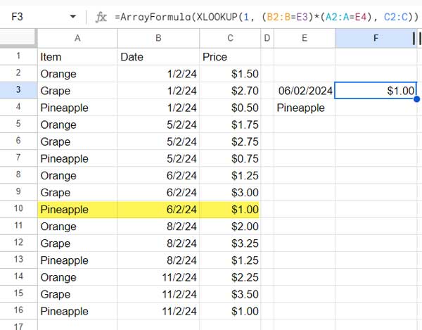
If you wish to hardcode the search keys, use the following formula instead:
=ArrayFormula(XLOOKUP(1, (B2:B=TODAY()) * (A2:A="Pineapple"), C2:C))The logical test B2:B=TODAY() evaluates to TRUE or FALSE in rows and similarly to A2:A="Pineapple". In any row where column B is equal to today’s date and column A is equal to “Pineapple”, the formula returns TRUE * TRUE, which is equal to 1. So we have used 1 as the search key in the XLOOKUP.
Note: These types of logical tests only apply to an exact match of the search key in XLOOKUP.
XLOOKUP for the Nearest Past Date to Today’s Date
Here is another example of using XLOOKUP with dates. We have seen how to look up today’s date with or without an item and retrieve the corresponding price. Now, let’s explore finding the price on the nearest past date to today.
Enter =TODAY() in cell E3 to use as the search key and enter this formula in cell F3:
=XLOOKUP(E3-1, B2:B, C2:C, ,-1)In this formula, we have deducted 1 day from today’s date. XLOOKUP searches that date in column B for an approximate match that is less than or equal to the search key and returns the price from column C.
The fifth argument is -1, which represents match mode for an exact match or the next value that is lesser than the search key.
What about finding the price of Pineapple on the nearest past date to today?
Here also, the search keys are in cells E3 and E4 as per the earlier example. Here we will use E3-1 (TODAY()-1) as the search key but omit using E4 (“Pineapple”). Instead, we will use E4 in the lookup range.
In the lookup range, we will use IF(A2:A=E4, B2:B) to return only the dates that match “Pineapple” in column A. The formula will look up the search key, i.e., E3-1, in this column, and you can anticipate the outcome.
=ArrayFormula(XLOOKUP(E3-1, IF(A2:A=E4, B2:B), C2:C, "", -1))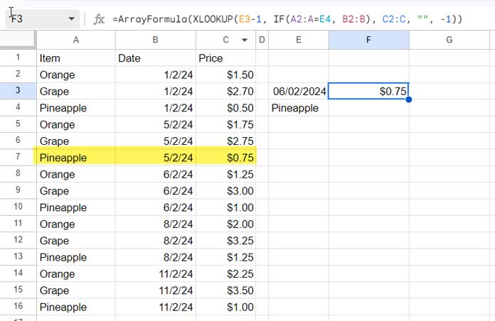
Note: These types of logical tests can apply to both approximate and exact matches of the search key in XLOOKUP.
This is another productive example of using XLOOKUP with dates in Google Sheets.
XLOOKUP for the Nearest Future Date to Today’s Date
Here you need to make two changes in the formula:
Replace the search key E3-1 with E3+1 and -1, which is the match mode, with 1.
=XLOOKUP(E3+1, B2:B, C2:C, ,1)The formula searches today’s+1 in column B or the next date that is greater than or equal to the search key.
To XLOOKUP the price of an item that is closest to today’s date, use the below formula.
=ArrayFormula(XLOOKUP(E3+1, IF(A2:A=E4, B2:B), C2:C, "", 1))Identifying the Last or First Occurrence of the Date Search Key
This is a common requirement. If you have multiple entries on the same date, you may want to look up the last or first entry.
Let’s find the first and last receipt of an item on 08 February 2024.
=XLOOKUP(DATE(2024, 2, 8), B2:B, A2:A, ,0, 1) // Returns the first occurrence
=XLOOKUP(DATE(2024, 2, 8), B2:B, A2:A, ,0, -1) // Returns the last occurrence
The sixth argument 1 searches from the first value to the last value, whereas -1 searches from the last value to the first value.
The date criterion (search key) is hard-coded in this XLOOKUP formula. The DATE function is employed, and the syntax is as follows: DATE(year, month, day).
Alternatively, you can enter the date in cell E3 and refer to that, as per previous examples.
XLOOKUP in a Timestamp Column
We have seen using XLOOKUP with a date in Google Sheets. What about looking up a date or timestamp in a timestamp column?
XLOOKUP Date in a Timestamp Column:
When it comes to looking up a date in a timestamp column, wrap the lookup range with the INT function, which will return dates from timestamps. However, you should enter the XLOOKUP formula as an array formula.
Example:
=ArrayFormula(XLOOKUP(DATE(2023, 9, 19), INT(A2:A), B2:B))XLOOKUP Timestamp in a Timestamp Column:
If you want to look up a timestamp, enter the timestamp in any cell and use that as the search key. You won’t encounter any issues. However, if you want to hardcode the search key, follow this example:
=ArrayFormula(XLOOKUP(DATE(2023, 9, 19)+TIME(9, 46, 14), A2:A, B2:B))Where the date component in the search key is as per the syntax DATE(year, month, day), and the time component in the search key is as per the syntax TIME(hour, minute, second).
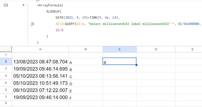
Addressing Timestamp with Milliseconds Issue:
If the timestamps include milliseconds, the above XLOOKUP formula would return #N/A (you won’t see the milliseconds unless you format the date column to DD/MM/YYYY HH:mm:ss.000).
So, you might want to replace A2:A (lookup range) with A2:A-QUERY(A2:A, "SELECT millisecond(A) LABEL millisecond(A)''", 0)/86400000, and the formula will become:
=ArrayFormula(
     XLOOKUP(
          DATE(2023, 9, 19)+TIME(9, 46, 14),
          A2:A-QUERY(A2:A, "Select millisecond(A) label millisecond(A)''", 0)/86400000,
          B2:B
     )
)
Related: How to Remove Milliseconds from Timestamps in Google Sheets
XLOOKUP in a Time Column
Assume we have employee check-in time recorded in Google Sheets where column A contains the date, column B contains the check-in time, and column C contains employee names.
To find who has first checked in, you can use the following formula:
=XLOOKUP(TIME(0, 0, 0), B2:B, C2:C, ,1)To find who has last checked in, the following formula will do the trick.
=XLOOKUP(TIME(23, 59, 59), B2:B, C2:C, ,-1)In both formulas, I’ve hardcoded the search key in the TIME function format TIME(hour, minute, second), which we have already seen in the timestamp examples. If you want, you can enter the search key 00:00:00 or 23:59:59 in a cell and refer to that in the formula.
Note: You can replace the criterion TIME(0, 0, 0) with MIN(B2:B) as well as TIME(23, 59, 59) with MAX(B2:B). While doing so, set the fifth argument to 0 instead of 1 or -1.
How do we find who has last checked in today?
You can use XLOOKUP with date and time as follows:
=ArrayFormula(XLOOKUP(TIME(23, 59, 59), IF(A2:A=TODAY(), B2:B,), C2:C, ,-1))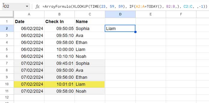
To find who has first checked in today, use the following formula.
=ArrayFormula(XLOOKUP(TIME(0, 0, 0), IF(A2:A=TODAY(), B2:B,), C2:C, ,1))Conclusion
The above examples effectively explain how to use XLOOKUP with date and time in Google Sheets.
For more XLOOKUP examples in Google Sheets, refer to our Complete Guide to XLOOKUP in Google Sheets.


