VLOOKUP vs XLOOKUP in Google Sheets: What’s the Difference and Which Should You Use?
This guide breaks down the main differences, strengths, and use cases of VLOOKUP and XLOOKUP so you can choose the right tool for your spreadsheet tasks.
If you want to explore more techniques like this, visit our Complete Guide to XLOOKUP in Google Sheets, where we compile practical XLOOKUP examples in Google Sheets ranging from beginner formulas to advanced lookup strategies.
Why Learn the Differences Between VLOOKUP and XLOOKUP?
Knowing the key differences between VLOOKUP and XLOOKUP in Google Sheets can help you:
- Choose the right function for your specific needs.
- Troubleshoot lookup errors more effectively.
- Understand limitations and capabilities to make better spreadsheet decisions.
Note: This guide focuses on the VLOOKUP and XLOOKUP key differences in Google Sheets, which may differ slightly from Excel.
Quick Comparison Table: VLOOKUP vs XLOOKUP in Google Sheets
| Feature / Difference | VLOOKUP | XLOOKUP |
| Lookup Direction | Vertical only | Vertical and horizontal |
| Column Limitation | Must search from first column only | Can search any column |
| Error Handling | Requires IFNA wrapper | Built-in error handler ([if_not_found]) |
| Exact/Approximate Match in Unsorted Data | Exact match only (with FALSE) | Multiple match modes (0, 1, -1, 2) |
| Reverse Lookup (Bottom to Top) | Not supported | Supported (search_mode = -1) |
| Handling Sorted Data (Asc/Desc) | Only ascending sort, limited flexibility | Full control with search_mode (2 for A→Z, -2 for Z→A) |
| Multiple Return Columns | Supports with {index1, index2, …} | Returns one-dimensional array only |
| Insertion-Safe | Not safe — column positions matter | Safe — uses separate lookup/result ranges |
| Ease of Use | Shorter syntax but less flexible | More readable, feature-rich |
Purpose of Lookup Functions in Google Sheets
All lookup functions retrieve data from a range based on a search key.
- VLOOKUP is limited to vertical lookups.
- XLOOKUP can perform both vertical and horizontal lookups, offering greater flexibility.
For horizontal lookups, Google Sheets also includes the HLOOKUP function, which works similarly to VLOOKUP but across rows instead of columns.
1. VLOOKUP vs XLOOKUP Syntax and Argument Differences
Release History:
- VLOOKUP has been available since Google Sheets launched in 2006.
- XLOOKUP was introduced in 2022 as a more advanced, flexible lookup tool.
Syntax Comparison:
VLOOKUP(search_key, range, index, [is_sorted])XLOOKUP(search_key, lookup_range, result_range, [missing_value], [match_mode], [search_mode])
Only the search_key argument is common. XLOOKUP replaces range and index with clearly defined lookup_range and result_range, and adds new options.
2. Flexible Lookup Ranges and Column Insert Safety
Sample Table: Least Populated Countries
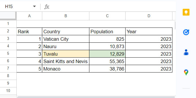
VLOOKUP Example:
=VLOOKUP("Tuvalu", B3:D7, 2, FALSE)- Searches “Tuvalu” in the first column of B3:D7
- Returns the value from the 2nd column
- Must specify
FALSEfor an exact match
XLOOKUP Example:
=XLOOKUP("Tuvalu", B3:B7, C3:C7)- Separates the lookup and return ranges
- No need to specify match mode for exact match (default behavior)
Why XLOOKUP Is Better Here:
- You can look up from any column, not just the leftmost one
- Safer against column insertions (no hard-coded index number)
Reverse Lookup Example (Find country by population):
=XLOOKUP(12829, C3:C7, B3:B7)VLOOKUP workaround:
=VLOOKUP(12829, {C3:C7, B3:B7}, 2, FALSE)Or using HSTACK:
=VLOOKUP(12829, HSTACK(C3:C7, B3:B7), 2, FALSE)3. Handling #N/A Errors More Elegantly with XLOOKUP
Scenario: Searching for a country not in the list, e.g., “Australia”
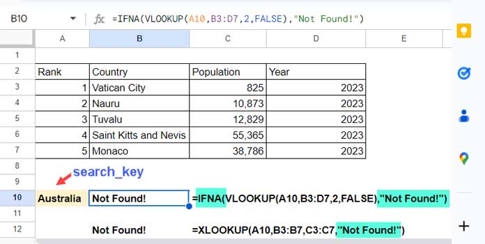
VLOOKUP:
=IFNA(VLOOKUP("Australia", B3:D7, 2, FALSE), "Not Found!")XLOOKUP: (built-in error handling)
=XLOOKUP("Australia", B3:B7, C3:C7, "Not Found!")VLOOKUP vs XLOOKUP Key Difference 1: XLOOKUP includes built-in IFNA functionality, reducing the need for nested formulas.
4. Exact and Approximate Matches in Unsorted Data
VLOOKUP:
- Can only perform exact matches in unsorted ranges when
is_sortedis set toFALSE
XLOOKUP:
- Supports multiple match modes:
0for exact match2for wildcard match (e.g., “Vatican*”)1for next largest match-1for next smallest match
Examples:
=XLOOKUP(1000, C3:C7, B3:B7, "Not Found!", -1) // returns "Vatican City"VLOOKUP vs XLOOKUP Key Difference 2: XLOOKUP allows approximate matches in unsorted ranges.
5. How to Use XLOOKUP for Bottom-to-Top (Reverse) Lookup
Unlike VLOOKUP, which always searches from top to bottom, XLOOKUP can search in the opposite direction — from bottom to top — by setting search_mode to -1. This is helpful when the lookup range contains multiple instances of a value and you want to return the last occurrence instead of the first.
Example:
=XLOOKUP("Tuvalu", B3:B7, C3:C7, , , -1)This formula searches for “Tuvalu” starting from the bottom of the range and returns the corresponding value from the same relative position in column C.
VLOOKUP vs XLOOKUP Key Difference 3: XLOOKUP can do reverse lookups; VLOOKUP cannot.
6. Lookup Behavior in Sorted Data
VLOOKUP:
- If
is_sorted = TRUE, data must be sorted A-Z - Approximate match returns the last lower value
- Exact match returns the last match
XLOOKUP:
- Can handle both ascending and descending sorted data using
search_mode = 2(A-Z) or-2(Z-A) - Exact match returns the first match
- Approximate match returns next smaller or next larger value based on
match_mode
VLOOKUP vs XLOOKUP Key Difference 4: XLOOKUP provides more control over sorted data lookup behavior.
7. VLOOKUP vs XLOOKUP: When VLOOKUP Is Still Better
Although XLOOKUP is more versatile in many ways, there are a few situations where VLOOKUP can be more convenient. One such case is when you want to return results from multiple columns at once for a set of search keys.
- XLOOKUP returns a one-dimensional array that matches the shape of the lookup range. If you pass a range with multiple lookup values, the result is vertical or horizontal accordingly, but only one column or row wide.
- VLOOKUP, on the other hand, allows you to return multiple columns at once by using an array constant like
{2,3,4}as the column index.
Example:
=ArrayFormula(VLOOKUP("Tuvalu", B3:D7, {1, 2, 3}, FALSE))This formula returns values from the 1st, 2nd, and 3rd columns for the match found in column B.
VLOOKUP vs XLOOKUP Key Difference 5: VLOOKUP can return multiple columns of results in one step using an index array. XLOOKUP only returns a one-dimensional array.
Conclusion: Choosing Between VLOOKUP and XLOOKUP in Google Sheets
If you’re still using VLOOKUP in Google Sheets, it’s time to consider switching. XLOOKUP is:
- Easier to read and write
- More flexible with lookup direction and error handling
- Safer against data structure changes
While both functions are supported, understanding the VLOOKUP vs XLOOKUP key differences ensures you’re using the best tool for your needs in Google Sheets.


