Sometimes we may require Xlookup Nth occurrence of a matching value in a table in Google Sheets. Is that possible?
Yep! The easiest way will be using a Filter and Index combination.
But you may lack the built-in Xlookup features such as wildcard use and search from top or bottom.
Assume there are country names in column A and some figures in column B.
We can use the following INDEX and FILTER combination formula to match the 3rd occurrence of the country name “USA” in column A and return the corresponding value from column B.
=index(filter(B:B,A:A="USA"),3)We can’t use “US*” with the above combo when we are unsure whether column A contains “US” or “USA.”
But the REGEXMATCH can come to our rescue.
=index(filter(B:B,regexmatch(A:A,"US")),3)Still, the other drawbacks (search from first or last) remain. Also, it may not support multiple search keys, e.g., “UK” and “USA,” in one go.
So let’s learn how to use Xlookup for matching the Nth occurrence of a value in Google Sheets.
We have three sets of formulas.
- Search from the first entry to the last entry.
- Search from the last entry to the first entry.
- Wildcards in Xlookup Nth Occurrence.
You only concentrate on the first set of formulas. Others will be easy for you to learn as they are much similar.
1. XLOOKUP Nth Match and Search from First to Last
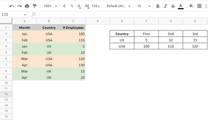
Our sample data is in columns A to C, and the criteria are in cell range E3:E4.
Please note that it isn’t necessary to use sorted data for Xlookup Nth match of a value in Google Sheets.

We have two criteria to match in the XLOOKUP function. They are “UK” and “USA” in cell range E3:E4 (vertically).
So the following formulas will return two values vertically. You can control the number of criteria by modifying E3:E4 in the Xlookup below.
F3 Formula (1st Occurrence):
=ArrayFormula(xlookup(E3:E4,B2:B,C2:C,"",0,1))It’s a regular formula that returns 5 and 100. Please refer to the image above.
G3 Formula (2nd Occurrence):
=ArrayFormula(xlookup(E3:E4, filter(B2:B, countifs(B2:B,B2:B,row(B2:B),"<="&row(B2:B))=2),filter(C2:C, countifs(B2:B,B2:B,row(B2:B),"<="&row(B2:B))=2),"",0,1))It returns 10 and 110.
H3 Formula (3rd Occurrence):
=ArrayFormula(xlookup(E3:E4, filter(B2:B, countifs(B2:B,B2:B,row(B2:B),"<="&row(B2:B))=3),filter(C2:C, countifs(B2:B,B2:B,row(B2:B),"<="&row(B2:B))=3),"",0,1))It returns 15 and 120.
If you compare G3 and H3 formulas, you can see that the only difference is in the highlighted parts. The number 2 in the G3 formula becomes 3 in H3.
Modify those parts to Xlookup Nth match of a value from the first entry to the last entry in Google Sheets.
Anatomy of the XLOOKUP Nth Match Formula
In the above example, let’s pick the G3 formula to learn since F3 is a regular Xlookup.
Regarding H3, it’s not different from G3. Only the Nth value varies in both.
So let’s learn the G3 formula step by step.
Syntax: XLOOKUP(search_key, lookup_range, result_range, [missing_value], [match_mode], [search_mode])
1. Search_key:
E3:E4
2. lookup_range:
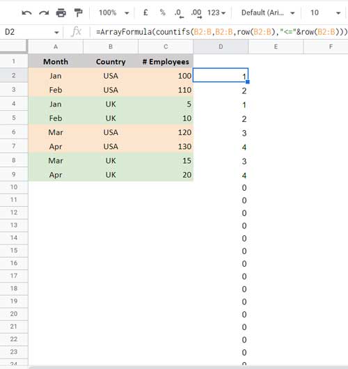
The following running count formula generates the running count of the occurrence of items in the Xlookup criteria field, which is column B.
=ArrayFormula(countifs(B2:B,B2:B,row(B2:B),"<="&row(B2:B)))I’ve entered it in cell D2 for your reference (we will use it within our Xlookup 2nd occurrence formula itself).

In the G3 formula, the Nth is equal to 2. So filter B2:B for the count of occurrence is equal to 2 to get the lookup_range for Xlookup
=filter(B2:B, countifs(B2:B,B2:B,row(B2:B),"<="&row(B2:B))=2)3. result_range:
To get the result_range, filter C2:C for the count of occurrence is equal to 2.
=filter(C2:C, countifs(B2:B,B2:B,row(B2:B),"<="&row(B2:B))=2)4. missing_value:
""
5. match_mode:
0
6. search_mode
1
That’s how we use Xlookup for the Nth match of a value from the first entry to the last entry in Google Sheets.
2. XLOOKUP Nth Match and Search from Last to First
Here are the changes you should make in the F3, G3, and H3 formulas to Xlookup Nth match from the last entry to the first entry.
In the F3 regular formula, replace 1 in the last part of it with -1.
In the other two, replace <= in the running count formula with >=. That means we require a reverse running count formula.
Replacing 1 with -1 is not a must here because of the filtered data. First and Last don’t make any difference.
3. Wildcards
The asterisk is one of the most common WILDCARDS. How to use it in Xlookup Nth occurrence match in Google Sheets?
The answer is how you use it in your regular formula.
For example, to Xlookup “US” instead of “USA,” you can use the F3 formula as given below.
=ArrayFormula(xlookup(E3:E4&"*",B2:B,C2:C,"",2,1))Note:- The criteria must be “US” in E3:E4. So it will match both “US” and “USA” in column B.
Added an asterisk with the criteria part and replaced 0 with 2 in the match_mode.
It applies to the 2nd, 3rd, and Nth occurrence Xlookup formulas.
That’s all. Thanks for the stay. Enjoy!


