This tutorial is all about getting the reverse count of occurrences of items in a list.
It’s called reverse running count, and I have a simplified version of an array formula that works perfectly in Google Sheets.
What do you mean by a simplified version?
Long back, I have shared an array formula for the same that is somewhat complex. You can find that here – Get the Count of Occurrences in Each Row in Google Sheets (Combo Formula).
Later, I have found out that it’s simple to transform a running count array formula to reverse running count.
I’ll explain how to do that below.
Example

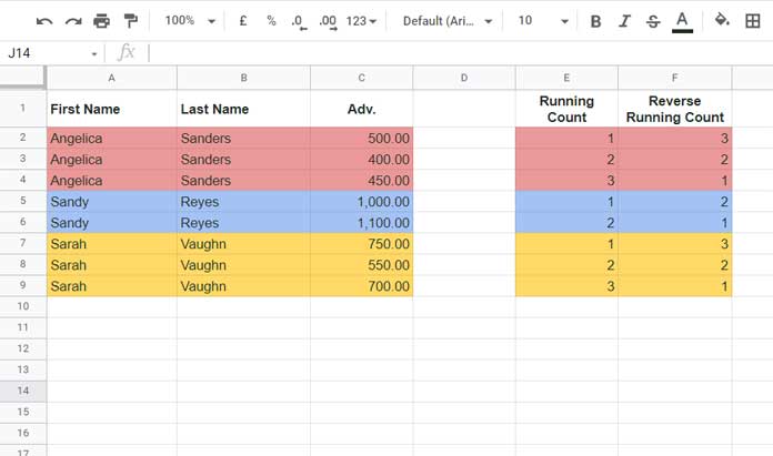
The above list (A1:C) contains three names in multiple occurrences, and they are “Angelica Sanders,” “Sandy Reyes,” and “Sarah Vaughn.”
Take a look at column F for the reverse count of occurrences of names in the list.
How do they come into use in a real-life scenario?
The reverse running count formula will be widely useful to filter the list in several ways.
Here are two FILTER function-based formulas.
With the formulas, I want to filter the advance amount taken by each person (column C) in the last/recent time.
If the list is arranged from oldest to newest, use the reverse running count column in the filter criteria.
=filter(A2:C9,F2:F9=1)Result:
| Angelica | Sanders | 450 |
| Sandy | Reyes | 1100 |
| Sarah | Vaughn | 700 |
On the contrary, if the list is arranged from newest to oldest, use the running count column in the filter criteria.
=filter(A2:C9,E2:E9=1)| Angelica | Sanders | 500 |
| Sandy | Reyes | 1000 |
| Sarah | Vaughn | 750 |
Array Formula for Reverse Running Count in Google Sheets
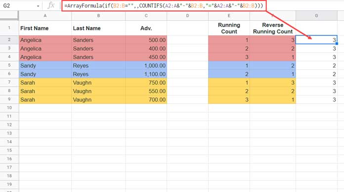
The simplified way to return the reverse running count in Google Sheets is to use COUNTIFS in array form. Here is how.
F2 Formula:
=ArrayFormula(
     if(
        B2:B="",,
        COUNTIFS(
           sort(row(B2:B),1,0),
           "<="&sort(row(B2:B),1,0),
           A2:A&"-"&B2:B,
           "="&A2:A&"-"&B2:B
        )
     )
)
In the above list, the duplicate names are in adjoining rows. I have just arranged the list likewise to make you understand what the formula returns.
Revrese Running Count – Formula Explanation
Other than COUNTIFS, the rest of the formula part is to restrict the formula fill. So I am ignoring that part in the explanation part below.
Syntax: COUNTIFS(criteria_range1, criterion1, [criteria_range2, …], [criterion2, …]).
criteria_range1 – sort(row(B2:B),1,0)
criterion1 – "<="&sort(row(B2:B),1,0)
criteria_range2 – A2:A&"-"&B2:B
criterion2 – "="&A2:A&"-"&B2:B
In this formula, criteria_range1 and criterion1 hold the key.
If you remove that, you will get the count of occurrence of names in each row. Not the running count in each row.
=ArrayFormula(if(B2:B="",,COUNTIFS(A2:A&"-"&B2:B,"="&A2:A&"-"&B2:B)))
The above reverse running count array formula works like this in Google Sheets.
It tests the list for duplicates of the strings (names) in two ways.
- The combined names (first and last names) are equal to the combined first and last names. That’s the creteria_range2 and criterion2.
- Then tests the reverse sorted row numbers are less than or equal to the reverse sorted row numbers. That’s the creteria_range1 and criterion1.
I know the first point doesn’t require any explanation.
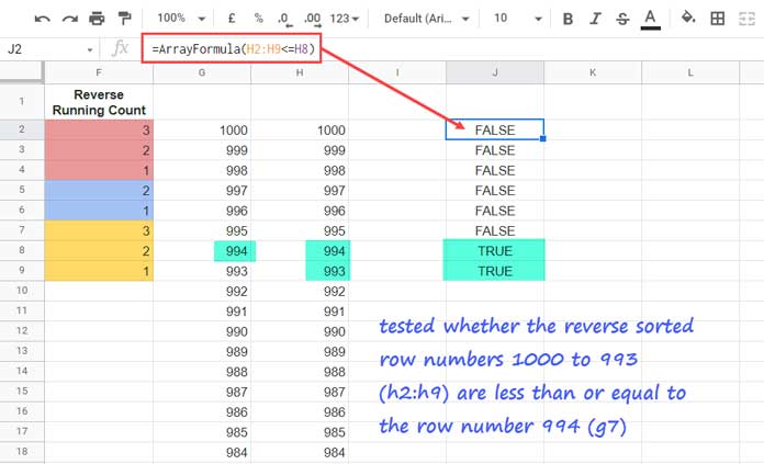
Regarding point 2, let’s test/compare a single row number (994) with the reverse sorted row numbers (1000 to 993).
Please see the following screenshot which is self-explanatory.

The formula returns TRUE up to the criterion from the bottom.
I hope that makes sense.
Update: The below formula will also work.
=ArrayFormula(
     if(
        B2:B="",,
        COUNTIFS(
           row(B2:B),
           ">="&row(B2:B),
           A2:A&"-"&B2:B,
           "="&A2:A&"-"&B2:B
        )
     )
)
Related Resources
- Reverse Running Total in Google Sheets (Array Formula).
- Array Formula for Conditional Running Total in Google Sheets.
- How to Calculate Running Balance in Google Sheets.
- Normal and Array Based Running Total Formula in Google Sheets.
- Cumulative Count of Distinct Values in Google Sheets (How-To).
- Cumulative Balance against Each Payment in Google Sheets.
- Sum, Count, Cumulative Sum Comma Separated Values in Google Sheets.


